Massachusetts Institute of Technology
6.042J/18.062J, Spring ’10: Mathematics for Computer Science
Prof. Albert R. Meyer
May 7
revised May 5, 2010, 857 minutes
Solutions to In-Class Problems Week 13, Fri.
Problem 1.
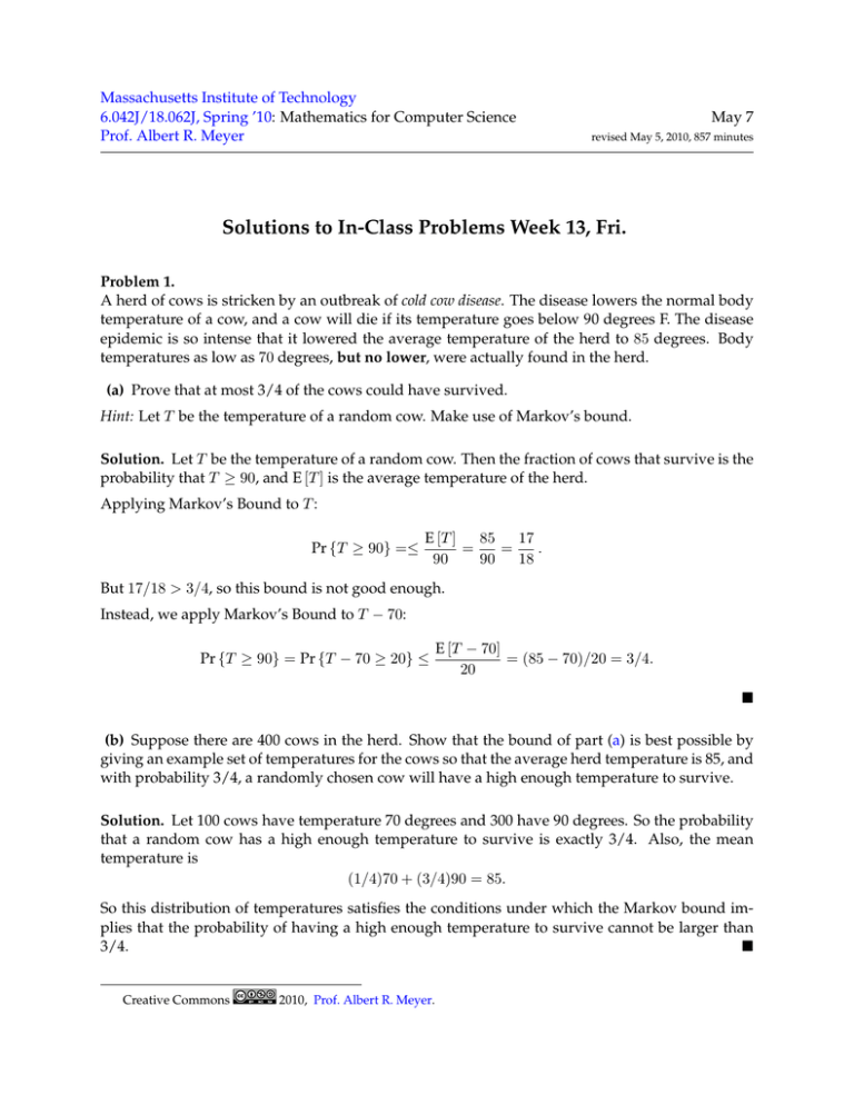
A herd of cows is stricken by an outbreak of cold cow disease. The disease lowers the normal body
temperature of a cow, and a cow will die if its temperature goes below 90 degrees F. The disease
epidemic is so intense that it lowered the average temperature of the herd to 85 degrees. Body
temperatures as low as 70 degrees, but no lower, were actually found in the herd.
(a) Prove that at most 3/4 of the cows could have survived.
Hint: Let T be the temperature of a random cow. Make use of Markov’s bound.
Solution. Let T be the temperature of a random cow. Then the fraction of cows that survive is the
probability that T ≥ 90, and E [T ] is the average temperature of the herd.
Applying Markov’s Bound to T :
Pr {T ≥ 90} =≤
E [T ]
85
17
=
=
.
90
90
18
But 17/18 > 3/4, so this bound is not good enough.
Instead, we apply Markov’s Bound to T − 70:
Pr {T ≥ 90} = Pr {T − 70 ≥ 20} ≤
E [T − 70]
= (85 − 70)/20 = 3/4.
20
�
(b) Suppose there are 400 cows in the herd. Show that the bound of part (a) is best possible by
giving an example set of temperatures for the cows so that the average herd temperature is 85, and
with probability 3/4, a randomly chosen cow will have a high enough temperature to survive.
Solution. Let 100 cows have temperature 70 degrees and 300 have 90 degrees. So the probability
that a random cow has a high enough temperature to survive is exactly 3/4. Also, the mean
temperature is
(1/4)70 + (3/4)90 = 85.
So this distribution of temperatures satisfies the conditions under which the Markov bound im­
plies that the probability of having a high enough temperature to survive cannot be larger than
3/4.
�
Creative Commons
2010, Prof. Albert R. Meyer.
2
Solutions to In-Class Problems Week 13, Fri.
Problem 2.
A gambler plays 120 hands of draw poker, 60 hands of black jack, and 20 hands of stud poker per
day. He wins a hand of draw poker with probability 1/6, a hand of black jack with probability
1/2, and a hand of stud poker with probability 1/5.
(a) What is the expected number of hands the gambler wins in a day?
Solution. 120(1/6) + 60(1/2) + 20(1/5) = 54.
�
(b) What would the Markov bound be on the probability that the gambler will win at least 108
hands on a given day?
Solution. The expected number of games won is 54, so by Markov, Pr {R ≥ 108} ≤ 54/108 =
1/2.
�
(c) Assume the outcomes of the card games are pairwise independent. What is the variance in
the number of hands won per day?
Solution. The variance can also be calculated using linearity of variance. For an individual hand
the variance is p(1 − p) where p is the probability of winning. Therefore the variance is
120(1/6)(5/6) + 60(1/2)(1/2) + 20(1/5)(4/5) = 523/15 = 34
13
15 .
�
(d) What would the Chebyshev bound be on the probability that the gambler will win at least
108 hands on a given day? You may answer with a numerical expression that is not completely
evaluated.
Solution.
Pr {R − 54 ≥ 54} ≤ Pr {|R − 54| ≥ 54} ≤
V ar[R]
523
=
≈ 0.01196.
2
15(54)2
54
(A very slightly better bound of 0.01182 comes from using the one-sided Chebyshev bound from
Problem ??.)
�
Problem 3.
The proof of the Pairwise Independent Sampling Theorem 21.5.1 was given for a sequence R1 , R2 , . . .
of pairwise independent random variables with the same mean and variance.
The theorem generalizes straighforwardly to sequences of pairwise independent random vari­
ables, possibly with different distributions, as long as all their variances are bounded by some
constant.
Solutions to In-Class Problems Week 13, Fri.
3
Theorem (Generalized Pairwise Independent Sampling). Let X1 , X2 , . . . be a sequence of pairwise
independent random variables such that Var [Xi ] ≤ b for some b ≥ 0 and all i ≥ 1. Let
X1 + X2 + · · · + Xn
,
n
µn ::= E [An ] .
An ::=
Then for every � > 0,
Pr {|An − µn | > �} ≤
b 1
· .
�2 n
(1)
(a) Prove the Generalized Pairwise Independent Sampling Theorem.
Solution. Essentially identical to the proof of Theorem 21.5.1 in the text, except that G gets re­
placed by X and Var [Gi ] by b, with the equality where the b is first used becoming ≤.
�
(b) Conclude that the following holds:
Corollary (Generalized Weak Law of Large Numbers). For every � > 0,
lim Pr {|An − µn | ≤ �} = 1.
n→∞
Solution.
Pr {|An − µn | ≤ �} =1 − Pr {|An − µn | > �}
≥1 − b/(n�2 )
and for any fixed �, this last term approaches 1 as n approaches infinity.
(by (1)),
�
MIT OpenCourseWare
http://ocw.mit.edu
6.042J / 18.062J Mathematics for Computer Science
Spring 2010
For information about citing these materials or our Terms of Use, visit: http://ocw.mit.edu/terms.