Continuous Expectation and Variance, the Law of Large Numbers, and the Central Limit Theorem
18.05
Spring 2014
Jeremy Orloff and Jonathan Bloom
0.5
0.4
0.3
0.2
0.1
0
-4 -3 -2 -1 0 1 2 3 4

Expected value
Expected value: measure of location, central tendency
X continuous with range [ a , b ] and pdf f ( x ):
� b
E ( X ) = xf ( x ) dx .
a
X discrete with values x
1
, . . . , x n and pmf p ( x i
): n n
E ( X ) = x i p ( x i
) .
i =1
View these as essentially the same formulas.
May 28, 2014 2 / 22

Variance and standard deviation
Standard deviation: measure of spread, scale
For any random variable X with mean µ
Var( X ) = E (( X − µ )
2
) , σ = Var( X )
X continuous with range [ a , b ] and pdf f ( x ): b
Var( X ) = ( x − µ )
2 a f ( x ) dx .
X discrete with values x
1
, . . . , x n and pmf p ( x i
): n n
Var( X ) = ( x i
− µ )
2 p ( x i
) .
i =1
View these as essentially the same formulas.
May 28, 2014 3 / 22

Properties
Properties:
1.
E ( X + Y ) = E ( X ) + E ( Y ).
2.
E ( aX + b ) = aE ( X ) + b .
1.
If X and Y are independent then
Var( X + Y ) = Var( X ) + Var( Y ).
2.
Var( aX + b ) = a 2 Var( X ).
3.
Var( X ) = E ( X 2 ) − E ( X ) 2 .
May 28, 2014 4 / 22

Board question
The random variable X has range [0,1] and pdf cx 2 .
a) Find c .
b) Find the mean, variance and standard deviation of X .
c) Find the median value of X .
d) Suppose X
1
, . . .
X
16 are independent identically-distributed copies of X .
Let X be their average.
What is the standard deviation of X ?
e) Suppose Y = X 4 .
Find the pdf of Y .
May 28, 2014 5 / 22

Quantiles
Quantiles give a measure of location.
φ ( z )
Area = prob. = .6
z
F ( q
.
6
) = .
6
1 q
.
6
= .
253
Φ( z ) z q
.
6
= .
253 q
.
6
: left tail area = .6
⇔ F ( q
.
6
) = .
6
May 28, 2014 6 / 22

Concept question
In each of the plots some densities are shown.
The median of the black plot is always at q p
.
In each plot, which density has the greatest median?
1.
Black 2.
Red
4.
All the same 5.
Impossible to tell
3.
Blue
May 28, 2014 7 / 22

Law of Large Numbers (LoLN)
Informally: An average of many measurements is more accurate than a single measurement.
Formally: Let X
1
, X
2
, .
.
.
be i.i.d.
random variables all with mean µ and standard deviation σ .
Let
X n
=
X
1
+ X
2
+ . . .
+ X n n
= n
1 n
X i
.
n i =1
Then for any (small number) a , we have lim P ( | X n
− µ | < a ) = 1 .
n →∞
May 28, 2014 8 / 22

Concept Question: Desperation
You have $100.
You need $1000 by tomorrow morning.
Your only way to get it is to gamble.
If you bet $k, you either win $k with probability p or lose $k with probability 1 − p .
Maximal strategy: Bet as much as you can, up to what you need, each time.
Minimal strategy: Make a small bet, say $5, each time.
1.
If p = .
45, which is the better strategy?
A.
Maximal B.
Minimal
May 28, 2014 9 / 22
2. If p = .
8, which is the better strategy?
A. Maximal B. Minimal

Concept Question: Desperation
You have $100.
You need $1000 by tomorrow morning.
Your only way to get it is to gamble.
If you bet $k, you either win $k with probability p or lose $k with probability 1 − p .
Maximal strategy: Bet as much as you can, up to what you need, each time.
Minimal strategy: Make a small bet, say $5, each time.
1.
If p = .
45, which is the better strategy?
A.
Maximal B.
Minimal
2.
If p = .
8, which is the better strategy?
A.
Maximal B.
Minimal
May 28, 2014 9 / 22

Histograms
2
1
4
3
Made by ‘binning’ data.
Frequency : height of bar over bin = number of data points in bin.
Density : area of bar is the fraction of all data points that lie in the bin.
So, total area is 1.
frequency density
0.4
0.3
0.2
0.1
.5
1.5
2.5
3.5
4.5
x
.5
1.5
2.5
3.5
4.5
x
May 28, 2014 10 / 22

Board question
1.
Make a both a frequency and density histogram from the data below.
Use bins of width 0.5
starting at 0.
The bins should be right closed.
1 1.2
1.3
1.6
1.6
2.1
2.2
2.6
2.7
3.1
3.2
3.4
3.8
3.9
3.9
2.
Same question using unequal width bins with edges 0, 1, 3, 4.
May 28, 2014 11 / 22

Solution
0 1 2 3 4 0 1 2 3 4
Histograms with equal width bins
0 1 2 3 4 0 1 2 3 4
Histograms with unequal width bins
May 28, 2014 12 / 22

LoLN and histograms
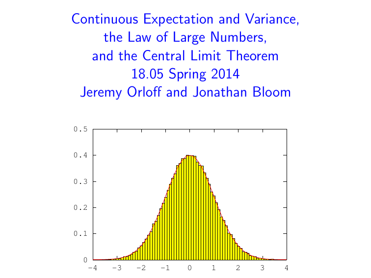
LoLN implies density histogram converges to pdf:
0.5
0.4
0.3
0.2
0.1
0
-4 -3 -2 -1 0 1 2 3 4
Histogram with bin width .1
showing 100000 draws from a standard normal distribution.
Standard normal pdf is overlaid in red.
May 28, 2014 13 / 22

Standardization
Random variable X with mean µ and standard deviation
σ .
Standardization: Z =
X − µ
.
σ
Z has mean 0 and standard deviation 1.
Standardizing any normal random variable produces the standard normal.
If X ≈ normal then standardized X ≈ stand.
normal.
May 28, 2014 14 / 22

Concept Question: Standard Normal
Normal PDF within 1 · σ ≈ 68% within 2 · σ ≈ 95% within 3 · σ ≈ 99%
68%
95%
99%
− 3 σ − 2 σ − σ σ 2 σ
1.
P ( − 1 < Z < 1) is a) .025
b) .16
c) .68
d) .84
e) .95
3 σ
2.
P ( Z > 2) a) .025
b) .16
c) .68
d) .84
e) .95
z
May 28, 2014 15 / 22

Central Limit Theorem
Setting: X
1
, X
2
, .
.
.
i.i.d.
with mean µ and standard dev.
σ .
For each n :
X n
1
= ( X n
1
+ X
2
+ . . .
+ X n
)
S n
= X
1
+ X
2
+ . . .
+ X n
.
Conclusion: For large n :
X n
�
≈ N µ,
σ n
2 �
S n
≈ N n µ, n σ
2
Standardized S n or X n
≈ N(0 , 1)
May 28, 2014 16 / 22

CLT: pictures
Standardized average of n i.i.d.
uniform random variables with n = 1 , 2 , 4 , 12.
0.5
0.4
0.35
0.3
0.25
0.2
0.15
0.1
0.05
0
-3 -2 -1 0 1 2 3
0.4
0.3
0.2
0.1
0
-3 -2 -1 0 1 2 3
0.4
0.35
0.3
0.25
0.2
0.15
0.1
0.05
0
-3
0.4
0.35
0.3
0.25
0.2
0.15
0.1
0.05
0
-3 -2 -1 0 1 2 3 -2 -1 0 1 2 3
May 28, 2014 17 / 22

CLT: pictures 2
The standardized average of n i.i.d.
exponential random variables with n = 1 , 2 , 8 , 64.
1 0.7
0.8
0.6
0.4
0.2
0
-3 -2 -1 0 1 2 3
0.6
0.5
0.4
0.3
0.2
0.1
0
-3 -2 -1 0 1 2 3
0.5
0.5
0.4
0.3
0.2
0.1
0
-3 -2 -1 0 1 2 3
0.4
0.3
0.2
0.1
0
-3 -2 -1 0 1 2 3
May 28, 2014 18 / 22

CLT: pictures 3
The standardized average of n i.i.d.
Bernoulli(.5) random variables with n = 1 , 2 , 12 , 64.
0.4
0.35
0.3
0.25
0.2
0.15
0.1
0.05
0
-3 -2 -1 0 1 2 3
0.4
0.35
0.3
0.25
0.2
0.15
0.1
0.05
0
-3 -2 -1 0 1 2 3
0.4
0.35
0.3
0.25
0.2
0.15
0.1
0.05
0
-3 -2 -1 0 1 2 3
0.4
0.35
0.3
0.25
0.2
0.15
0.1
0.05
0
-4 -3 -2 -1 0 1 2 3 4
May 28, 2014 19 / 22

CLT: pictures 4
The (non-standardized) average of n Bernoulli(.5) random variables, with n = 4 , 12 , 64.
(Spikier.)
1.4
3
1.2
1
0.8
0.6
0.4
0.2
0
-1 -0.5
0 0.5
1 1.5
2
2.5
2
1.5
1
0.5
0
-0.2
0 0.2 0.4 0.6 0.8
1 1.2 1.4
7
6
5
4
3
2
1
0
-0.2
0 0.2
0.4
0.6
0.8
1 1.2
1.4
May 28, 2014 20 / 22

Table Question: Sampling from the standard normal distribution
As a table, produce a single random sample from (an approximate) standard normal distribution.
The table is allowed nine rolls of the 10-sided die.
Note: µ = 5 .
5 and σ
2
= 8 .
25 for a single 10-sided die.
Hint: CLT is about averages.
May 28, 2014 21 / 22

Board Question: CLT
1.
Carefully write the statement of the central limit theorem.
2.
To head the newly formed US Dept.
of Statistics, suppose that 50% of the population supports Erika, 25% supports Ruthi, and the remaining 25% is split evenly between Peter, Jon and Jerry.
A poll asks 400 random people who they support.
What is the probability that at least 55% of those polled prefer
Erika?
3.
What is the probability that less than 20% of those polled prefer Ruthi?
May 28, 2014 22 / 22

0,72SHQ&RXUVH:DUH
KWWSRFZPLWHGX
,QWURGXFWLRQWR3UREDELOLW\DQG6WDWLVWLFV
6SULQJ
)RULQIRUPDWLRQDERXWFLWLQJWKHVHPDWHULDOVRURXU7HUPVRI8VHYLVLW KWWSRFZPLWHGXWHUPV