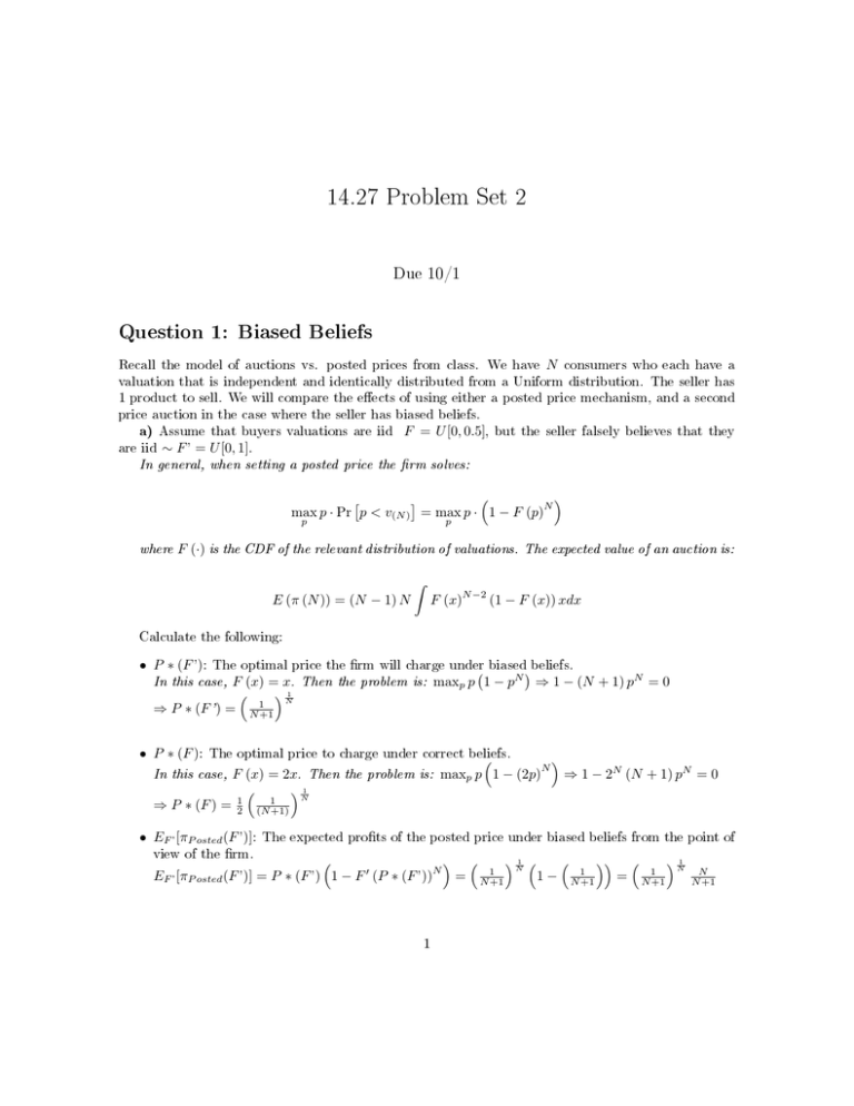
14.27 Problem Set 2
Due 10/1
Question 1: Biased Beliefs
Recall the model of auctions vs. posted prices from class. We have N consumers who each have a
valuation that is independent and identically distributed from a Uniform distribution. The seller has
1 product to sell. We will compare the eects of using either a posted price mechanism, and a second
price auction in the case where the seller has biased beliefs.
a) Assume that buyers valuations are iid F = U [0, 0.5], but the seller falsely believes that they
are iid ∼ F ' = U [0, 1].
In general, when setting a posted price the rm solves:
N
max p · Pr p < v(N ) = max p · 1 − F (p)
p
p
where F (·) is the CDF of the relevant distribution of valuations. The expected value of an auction is:
ˆ
E (π (N )) = (N − 1) N
N −2
F (x)
(1 − F (x)) xdx
Calculate the following:
• P ∗ (F '): The optimal price the rm will charge under biasedbeliefs.
In this case, F (x) = x. Then the problem is: maxp p 1 − pN ⇒ 1 − (N + 1) pN = 0
N1
⇒ P ∗ (F ') = N1+1
• P ∗ (F ): The optimal price to charge under correct beliefs.
In this case, F (x) = 2x. Then the problem is: maxp p 1 − (2p)N ⇒ 1 − 2N (N + 1) pN = 0
N1
⇒ P ∗ (F ) = 12 (N1+1)
• EF ' [πP osted (F ')]: The expected prots of the posted price under biased beliefs from the point of
view of the rm.
N1 N1
N
1 − N1+1
= N1+1
EF [πP osted (F ')] = P ∗ (F ') 1 − F 0 (P ∗ (F '))
= N1+1
'
1
N
N +1
N
Biased
Price
Optimal
Price
2
3
4
5
6
7
8
9
10
11
12
13
14
15
16
17
18
19
20
0.69
0.71
0.72
0.74
0.76
0.77
0.78
0.79
0.80
0.81
0.82
0.83
0.83
0.84
0.85
0.85
0.86
0.86
0.87
0.35
0.35
0.36
0.37
0.38
0.39
0.39
0.40
0.40
0.41
0.41
0.41
0.42
0.42
0.42
0.43
0.43
0.43
0.43
Posted Price
Auction
Expected
True Profits,
Expected
Expected
True Profits,
Profits,
Optimal
Profits, Biased Profits, Correct
Biased Price
Biased Price
Price
Beliefs
Beliefs
0.46
0
0.17
0.33
0.17
0.53
0
0.18
0.50
0.25
0.58
0
0.18
0.60
0.30
0.62
0
0.19
0.67
0.33
0.65
0
0.19
0.71
0.36
0.67
0
0.19
0.75
0.38
0.70
0
0.20
0.78
0.39
0.71
0
0.20
0.80
0.40
0.73
0
0.20
0.82
0.41
0.75
0
0.20
0.83
0.42
0.76
0
0.21
0.85
0.42
0.77
0
0.21
0.86
0.43
0.78
0
0.21
0.87
0.43
0.79
0
0.21
0.88
0.44
0.80
0
0.21
0.88
0.44
0.80
0
0.21
0.89
0.44
0.81
0
0.21
0.89
0.45
0.82
0
0.22
0.90
0.45
0.82
0
0.22
0.90
0.45
Figure 1: Prot Comparison
• EF [πP osted (F ')]: The expected prots of the posted price under biased beliefs but from the point
of view of what will actually happen.
N
N
EF [πP osted (F ')] = P ∗ (F 0 ) 1 − F (P ∗ (F '))
= P ∗ (F 0 ) max 1 − (2P ∗ (F 0 )) , 0
=
1
(N +1)
N1
max 1 −
2N
(N +1) , 0
• EF 0 [πAuction ]: The expected
rm.
´ prots from the auction from the
´ point of view of the
−1
EF 0 [πAuction ] = (N − 1) N xN −2 (1 − x) xdx = (N − 1) N xN −1 − xN dx = N
N +1
• EF [πAuction ] The actual expected prots from the auction.
In this case, f (x) = 2 and ´F (x) = 2x. Then:
´ 0.5 N −1
N −2
EF 0 [πAuction ] = (N − 1) N 2 (2x)
(1 − 2x) xdx = 2N −1 (N − 1) N 0
x
− 2xN dx
h N
i
N +1 0.5
−1
= 2N −1 (N − 1) N xN − 2 xN +1
= 12 N
N +1
0
Analyze the relation between all of these expected prots as a function of N , the number of bidders. It
may be useful to create a table as we did in class plotting the value for dierent values of N . Identify
when the rm chooses to use a posted price vs. an auction: does that always work out well for the
rm?
Note that the true prots under the biased optimal price are always 0! This is in contrast to the
2
auction, where under true and biased beliefs prots are always positive. The rm chooses an auction
for N ≥ 4, and really should pick an auction for N ≥ 3.
b) Repeat the exercise above using F ' = U [0, 2].
• P ∗ (F '): The optimal price the rm will charge under biased beliefs.
N In this case, F (x) = 21 x. Then the problem is: maxp p 1 − p2
⇒1−
N1
⇒ P ∗ (F ') = 2 N1+1
(N +1) N
p
2N
=0
• EF ' [πP osted (F ')]: The expected prots of the posted price under biased beliefs from the point of
view of the rm.
N1 N
N
EF [πP osted (F ')] = P ∗ (F ') 1 − F 0 (P ∗ (F '))
= 2 N1+1
N +1
'
• EF [πP osted (F ')]: The expected prots of the posted price under biased beliefs but from the point
of view of what will actually happen.
N1
N
EF [πP osted (F ')] = P ∗ (F 0 ) 1 − F (P ∗ (F '))
= 2 (N1+1)
max 1 − 4N N1+1 , 0
• EF 0 [πAuction ]: The expected prots from the auction from the point of view of the rm.
N −1 ´ 2 N −1 xN
´2
x
− 2 dx
EF 0 [πAuction ] = (N − 1) N 0 x2 N −2 1 − x2 x 12 dx = (N − 1) N 12
0
N −1
= 2 N +1
• EF [πAuction ] The actual expected prots from the auction.
These do not change:
1 N −1
2 N +1
3
N
Biased
Price
Optimal
Price
2
3
4
5
6
7
8
9
10
11
12
13
14
15
16
17
18
19
20
1.39
1.41
1.45
1.48
1.51
1.54
1.57
1.59
1.61
1.63
1.64
1.66
1.67
1.68
1.69
1.70
1.71
1.72
1.73
0.69
0.71
0.72
0.74
0.76
0.77
0.78
0.79
0.80
0.81
0.82
0.83
0.83
0.84
0.85
0.85
0.86
0.86
0.87
Posted Price
Auction
Expected
True Profits,
Expected
Expected
True Profits,
Profits,
Optimal
Profits, Biased Profits, Correct
Biased Price
Biased Price
Price
Beliefs
Beliefs
0.92
0
0.35
0.67
0.33
1.06
0
0.35
1.00
0.50
1.16
0
0.36
1.20
0.60
1.24
0
0.37
1.33
0.67
1.30
0
0.38
1.43
0.71
1.35
0
0.39
1.50
0.75
1.39
0
0.39
1.56
0.78
1.43
0
0.40
1.60
0.80
1.46
0
0.40
1.64
0.82
1.49
0
0.41
1.67
0.83
1.52
0
0.41
1.69
0.85
1.54
0
0.41
1.71
0.86
1.56
0
0.42
1.73
0.87
1.58
0
0.42
1.75
0.88
1.59
0
0.42
1.76
0.88
1.61
0
0.43
1.78
0.89
1.62
0
0.43
1.79
0.89
1.64
0
0.43
1.80
0.90
1.65
0
0.43
1.81
0.90
Figure 2: Prot Comparison
4
MIT OpenCourseWare
http://ocw.mit.edu
14.27 Economics and E-Commerce
Fall 2014
For information about citing these materials or our Terms of Use, visit: http://ocw.mit.edu/terms.