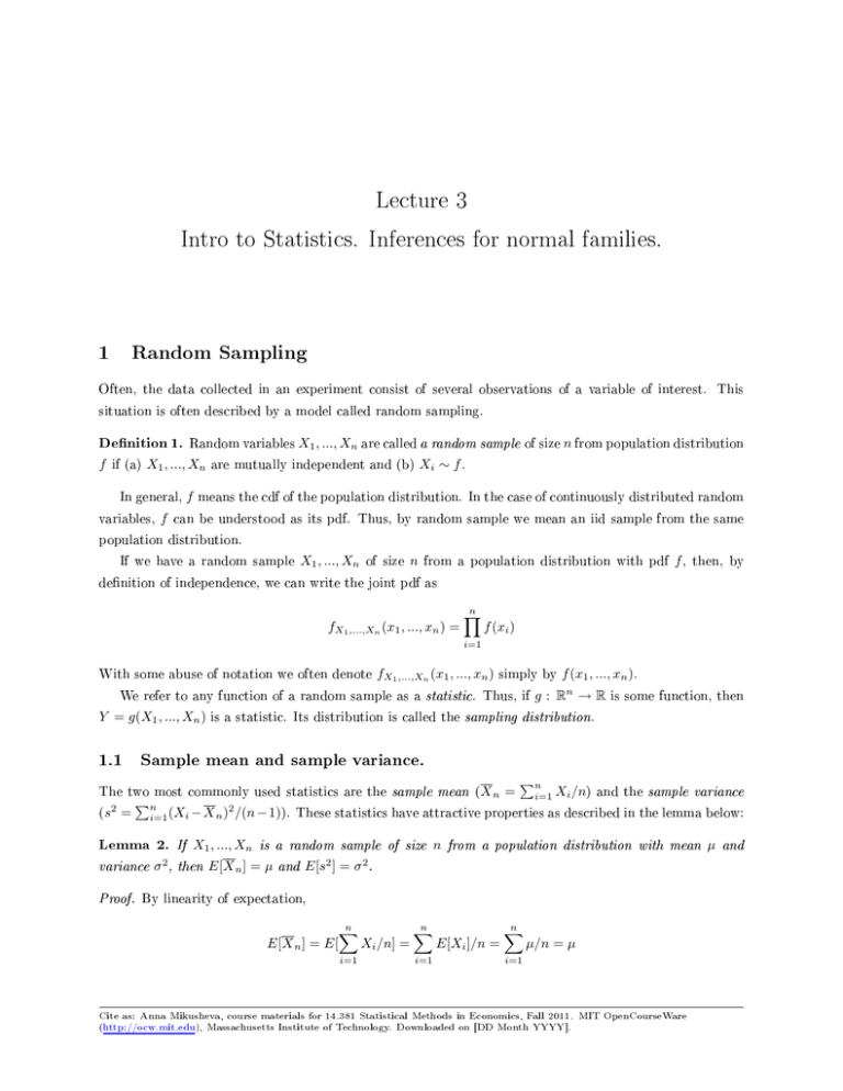
Lecture 3
Intro to Statistics. Inferences for normal families.
1 Random Sampling
Often, the data collected in an experiment consist of several observations of a variable of interest. This
situation is often described by a model called random sampling.
Denition 1. Random variables X1 , ..., Xn are called a random sample of size n from population distribution
f if (a) X1 , ..., Xn are mutually independent and (b) Xi ∼ f .
In general, f means the cdf of the population distribution. In the case of continuously distributed random
variables, f can be understood as its pdf. Thus, by random sample we mean an iid sample from the same
population distribution.
If we have a random sample X1 , ..., Xn of size n from a population distribution with pdf f , then, by
denition of independence, we can write the joint pdf as
fX1 ,...,Xn (x1 , ..., xn ) =
n
Y
f (xi )
i=1
With some abuse of notation we often denote fX1 ,...,Xn (x1 , ..., xn ) simply by f (x1 , ..., xn ).
We refer to any function of a random sample as a statistic. Thus, if g : Rn → R is some function, then
Y = g(X1 , ..., Xn ) is a statistic. Its distribution is called the sampling distribution.
1.1 Sample mean and sample variance.
Pn
The two most commonly used statistics are the sample mean (X n = i=1 Xi /n) and the sample variance
Pn
(s2 = i=1 (Xi − X n )2 /(n − 1)). These statistics have attractive properties as described in the lemma below:
Lemma 2. If X1 , ..., Xn is a random sample of size n from a population distribution with mean µ and
variance σ 2 , then E[X n ] = µ and E[s2 ] = σ 2 .
Proof. By linearity of expectation,
E[X n ] = E[
n
X
i=1
Xi /n] =
n
X
i=1
E[Xi ]/n =
n
X
µ/n = µ
i=1
Cite as: Anna Mikusheva, course materials for 14.381 Statistical Methods in Economics, Fall 2011. MIT OpenCourseWare
(http://ocw.mit.edu), Massachusetts Institute of Technology. Downloaded on [DD Month YYYY].
To show the second part of the lemma, denote Yi = Xi − µ and Y n =
Thus,
E[Yi2 ]
2
Pn
i=1
Yi /n. Note that E[Yi ] = 0.
2
= V (Yi ) = V (Xi ) = σ and V (Y n ) = σ /n. Then
E[s2 ] =
n
X
E[ (Xi − X n )2 /(n − 1)]
i=1
=
n
X
E[ ((Xi − µ) − (X n − µ))2 /(n − 1)]
=
n
X
E[ (Yi − Y n )2 /(n − 1)]
=
n
X
2
E [ (Yi2 − 2Yi Y n + Y n )]/(n − 1)
=
n
X
2
2
E[
Yi2 − 2nY n + nY n ]/(n − 1)
=
n
X
2
E[
Yi2 − nY n ]/(n − 1)
=
n
X
2
(
E[Yi2 ] − nE[Y n ])/(n − 1)
=
(nσ 2 − σ 2 )/(n − 1)
=
σ2
i=1
i=1
i=1
i=1
i=1
i=1
1.2 Empirical Distribution Function
If we have a random sample X1 , ..., Xn of size n, then empirical distribution function F̂n is the cdf of the
distribution that puts mass 1/n at each data point Xi . Thus, by denition,
F̂n (x) =
n
X
I(Xi ≤ x)/n,
i=1
where I(·) stands for the indicator function, i.e. the function which equals 1 if the statement in brackets is
true, and 0 otherwise. In other words, F̂n (x) shows the fraction of observations with a value smaller or equal
than x. An important property of an empirical distribution function is given in the lemma below.
Lemma 3. If we have a random sample X1 , ..., Xn of size n from a distribution with cdf F , then for any
x ∈ R, E[F̂n (x)] = F (x) and V (F̂n (x)) → 0 as n → ∞. As a consequence, F̂n (x) → F (x) in L2 and
F̂n (x) →p F (x) as n → ∞.
Proof. Note that I(Xi ≤ x) equals 1 with probability P {X ≤ x} and 0 otherwise. Thus, E[I(Xi ≤ x)] =
P {X ≤ x} = F (x). Hence E[F̂n (x)] = F (x) by linearity of expectation. In addition, V (I(Xi ≤ x)) =
2
F (x)(1 − F (x)) by the formula for variance of a Bernoulli (F (x)) distribution. Therefore,
V (F̂n (x)) =
n
X
V (I(Xi ≤ x))/n2 = F (x)(1 − F (x))/n → 0
i=1
To prove the second part of the lemma, we haveE[(F̂n (x) − F (x))2 ] = V (F̂n (x)) → 0 as n → ∞ since
E[F̂n (x)] = F (x). Convergence in probability then follows from convergence in quadratic mean.
Actually a much more strong result holds as well:
Theorem 4 (Glivenko-Cantelli). If X1 , ..., Xn is a random sample from a distribution with cdf F , then
sup |Fˆn (x) − F (x)| →p 0
x∈R
(and almost surely).
1.3 Plug-in estimators
Suppose we have a random sample X1 , ..., Xn of size n from population distribution with cdf F . Suppose T is
some function on the space of possible cdfs. Suppose we do not know F but we are interested in T (F ). Then
we can use some statistic g(X1 , ..., Xn ) to estimate T (F ). In this case g(X1 , ..., Xn ) is called an estimator
of T (F ). Its realization g(x1 , ..., xn ) is called an estimate of T (F ). Here x1 , ..., xn stand for realizations of
X1 , ..., Xn . What is a good estimator of T (F )? By common sense, a good estimator g(X1 , ..., Xn ) should be
such that g(X1 , ..., Xn ) ≈ T (F ), at least with large probability. One possible estimator is T (F̂n ) where F̂n
is the empirical cdf. T (F̂n ) is called a plug-in estimator. From the Glivenko-Cantelli theorem we know that
F̂n will be close to F with large probability in large samples. Thus, if T is continuous, then T (F̂n ) will be
close to T (F ).
As an example, suppose we are interested in the mean of the population distribution, i.e. µ = T (F ) =
R +∞
E[X] = −∞ xdF (x).Then
Z
+∞
µ̂ = T (F̂n ) =
xdF̂n (x) =
X
Xi /n = X n .
−∞
Thus, the plug-in estimator of the population mean is just the sample average. Next, suppose we are
R +∞
interested in the variance of the population distribution, i.e. σ 2 = T (F ) = E[(X − E[X])2 ] = −∞ (x −
3
R +∞
−∞
xdF (x))2 dF (x). Then
σ̂ 2
=
=
T (F̂n )
Z +∞
Z
(x −
−∞
Z +∞
=
=
+∞
xdF̂n (x))2 dF̂n (x)
−∞
(x − X n )2 dF̂n (x)
−∞
n
X
(Xi − X n )2 /n
i=1
Thus, the plug-in estimator of the population variance does not coincide with the sample variance. The
reason we use n − 1 in the denominator of the sample variance instead of n is to make it unbiased for the
population variance, i.e. E[s2 ] = σ 2 . Note that E[σ̂ 2 ] = (n − 1)σ 2 /n 6= σ 2 .
Finally, consider the plug-in estimator of quantiles. We already dened quantile of the distribution in
lecture 1 as qp = inf{x : F (x) ≥ p} so that qp is the p-th quantile of distribution F . Thus, plug-in estimator
of the p-th quantile is q̂p = inf{x : F̂n (x) ≥ p}.
1.4 Order Statistics
Let X1 , ..., Xn be a random sample from some distribution F . Let us order elements of X1 , ..., Xn such that
X(1) ≤ X(2) ≤ ... ≤ X(n) . Thus, X(1) is the minimal element among X1 , ..., Xn and X(n) is the maximal one.
In general, X(i) for all i = 1, ....n are called order statistics. X(n) − X(1) is called the sample range. Xdn/2e is
called the sample median. Here dxe denotes the smallest integer larger than x. Thus, Xdn/2e = q̂1/2 , i.e. the
sample median equals plug-in estimator of 1/2-th quantile. Xdn/4e is called the lower quartile and Xd3n/4e
the upper quartile. Finally, Xd3n/4e − Xdn/4e is the interquartile range.
The theorem below shows how one can calculate the density of order statistics.
Theorem 5. Let X1 , ..., Xn be a random sample from a distribution with cdf F and pdf f . Then the pdf of
X(j) is
fj (x) =
n!
f (x)(F (x))j−1 (1 − F (x))n−j
(j − 1)!(n − j)!
for all j = 1, ..., n.
Proof. By denition of order statistics, the cdf of X(j) is
Fj (x)
= P {X(j) ≤ x}
= P {at least j observations ≤ x}
n
X
=
P {exactly i observations ≤ x}
i=j
=
n
X
{n!(F (x))i (1 − F (x))n−i /(i!(n − i)!)}
i=j
4
Dierentiating Fj (x) yields
fj (x) =
=
dFj (x)/dx
n
X
{n!(F (x))i−1 (1 − F (x))n−i f (x)/((i − 1)!(n − i)!)}
i=j
−
n
X
{n!(F (x))i (1 − F (x))n−i−1 f (x)/(i!(n − i − 1)!)}
i=j
=
−
n
X
{n!(F (x))i−1 (1 − F (x))n−i f (x)/((i − 1)!(n − i)!)}
i=j
n
X
{n!(F (x))k−1 (1 − F (x))n−k f (x)/((k − 1)!(n − k)!)}
k=j+1
=
n!(F (x))j−1 (1 − F (x))n−j f (x)/((j − 1)!(n − j)!)
As an example, let X1 , ..., Xn be a random sample from U [0, 1]. Then f (x) = 1 if x ∈ [0, 1] and 0
otherwise. Thus, F (x) = 0 if x < 0, F (x) = x if x ∈ [0, 1], and F (x) = 1 otherwise. By the theorem above,
fj (x) = n!xj−1 (1 − x)n−j /((j − 1)!(n − j)!)
if x ∈ [0, 1] and fj (x) = 0 otherwise. So, by elementary algebra, E[X(j) ] =
R1
0
xfj (x)dx = j/(n + 1) and
2
V (X(j) ) = j(n − j + 1)/((n + 1) (n + 2)).
2 Parametric Families: Normal
The plug-in estimator considered above is a generic nonparametric estimator of some function T (F ) of
distribution F in the sense that it does not use any information about the class of possible distributions.
However, in practice, it is often assumed that the class of possible distributions form some parametric family.
In other words, it is assumed that F = F (θ) with θ ∈ Θ where Θ is some nite-dimensional set. Then θ
is called a parameter and Θ is a parameter space. In this case the cdf F and the corresponding pdf f are
often denoted by F (x|θ) and f (x|θ). If X1 , ..., Xn is a random sample from a distribution with pdf f (x|θ),
Qn
then joint pdf f (x1 , ..., xn |θ) = i=1 f (xi |θ). For xed x1 , ..., xn , f (x1 , ..., xn |θ) as a function of θ is called
the likelihood function.
One of the most important parametric families is a normal family when θ = (µ, σ 2 ) and the population
distribution is N (µ, σ 2 ). Before considering normal family, let us give some denitions related to normal
distributions.
If X1 , ..., Xn is a random sample from N (0, 1), then random variable χ2n =
Pn
i=1
Xi2 is called a χ2 random
2
variable with n degrees of freedom. Its distribution is called a χ distribution with n degrees of freedom.
It is known that its pdf is given by f (x) = xp/2−1 e−x/2 /(Γ(p/2)2p/2 ) if x > 0 and 0 otherwise. Here Γ(x)
denotes the gamma function. Its values can be found in special tables.
5
p
Next, if X0 is N (0, 1) and independent of X1 , ..., Xn , then tn = X0 / χ2n /n is called a t random variable
with n degrees of freedom. Its distribution is called a t-distribution or a Student distribution.
Finally, if χ2n and χ2m are independent χ2 random variables with n and m degrees of freedom correspondingly, then Fn,m = (χ2n /n)/(χ2m /m) is called a Fisher random variable with (n, m) degrees of freedom. Its
distribution is called a Fisher distribution with (n, m) degrees of freedom.
The following theorem gives some basic facts about the sample mean and the sample variance for random
sample from normal distribution:
Theorem 6. If X1 , ..., Xn are iid random variables with N (µ, σ 2 ) distribution, then (1) X n and sn2 are
independent, (2) X n ∼ N (µ, σ 2 /n), and (3) (n − 1)s2 /σ 2 ∼ χ2n−1 .
Proof. Let Z = X n , Y1 = X1 − X n , Y2 = X2 − X n , ..., Yn = Xn − X n . Then Z, Y1 , ..., Yn are jointly normal.
Obviously, E[Z] = µ and E[Yi ] = µ − µ = 0 for all i = 1, ..., n. In addition, V (Z) = σ 2 /n. Thus statement
(2) holds.
For any j = 1, ..., n,
cov(Z, Yj ) =
cov(X n , Xj − X n )
=
cov(X n , Xj ) − V (X n )
=
σ 2 /n − σ 2 /n
=
0
Since uncorrelated jointly normal random variables are independent, we conclude that Z is independent of
Pn
Pn
Y1 , Y2 , ..., Yn . Moreover, s2 = i=1 (Xi − X n )2 /(n − 1) = i=1 Yi2 /(n − 1) and statement (1) holds since
any functions of independent random variables are independent as well.
The proof of statement (3) is left for Problem set 1.
√
By denition, t = (X n − µ)/(s/ n) is called the t-statistic. Using the theorem above,
t=
Xn − µ
X −µ
1
N (0, 1)
√ = n√ p
∼q
= tn−1
s/ n
σ/ n
2
s2 /σ 2
χn−1 /(n − 1)
since N (0, 1) and χ2n−1 in the display above are independent. Thus, we proved that if X1 , ..., Xn is a random
sample from N (µ, σ 2 ), then t-statistic has t-distribution with n − 1 degrees of freedom.
Finally, let X1 , ..., Xn be a random sample from N (µx , σx2 ) and Y1 , ..., Ym be a random sample from
N (µy , σy2 ). Assume that X1 , ..., Xn are independent of Y1 , ..., Ym . Then F = (sx2 /sy2 )/(σx2 /σy2 ) is called a
F -statistic. Using the theorem above,
F =
s2x /s2y
χ2n−1 /(n − 1)
∼
= Fn−1,m−1
2
σx2 /σy2
χm−1
/(m − 1)
Thus, the F -statistic has the F -distribution with (n − 1, m − 1) degrees of freedom.
6
MIT OpenCourseWare
http://ocw.mit.edu
14.381 Statistical Method in Economics
Fall 2013
For information about citing these materials or our Terms of Use, visit: http://ocw.mit.edu/terms.