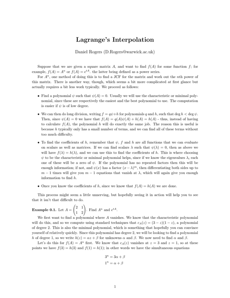
Lagrange’s Interpolation
Daniel Rogers (D.Rogers@warwick.ac.uk)
Suppose that we are given a square matrix A, and want to find f (A) for some function f ; for
example, f (A) = An or f (A) = etA . the latter being defined as a power series.
For An , one method of doing this is to find a JCF for the matrix and work out the nth power of
this matrix. There is another way, though, which seems a bit more complicated at first glance but
actually requires a bit less work typically. We proceed as follows:
• Find a polynomial ψ such that ψ(A) = 0. Usually we will use the characteristic or minimal polynomial, since these are respectively the easiest and the best polynomial to use. The computation
is easier if ψ is of low degree.
• We can then do long division, writing f = qψ+h for polynomials q and h, such that deg h < deg ψ.
Then, since ψ(A) = 0 we have that f (A) = q(A)ψ(A) + h(A) = h(A) - thus, instead of having
to calculate f (A), the polynomial h will do exactly the same job. The reason this is useful is
because h typically only has a small number of terms, and we can find all of these terms without
too much difficulty.
• To find the coefficients of h, remember that ψ, f and h are all functions that we can evaluate
on scalars as well as matrices. If we can find scalars λ such that ψ(λ) = 0, then as above we
will have f (λ) = h(λ), and we can use this to find the coefficients of h. This is where choosing
ψ to be the characteristic or minimal polynomial helps, since if we know the eigenvalues λi each
one of these will be a zero of ψ. If the polynomial has no repeated factors then this will be
enough information; if not, and ψ(x) has a factor (x − λ)m , then differentiating both sides up to
m − 1 times will give you m − 1 equations that vanish at λ, which will again give you enough
information to find h.
• Once you know the coefficients of h, since we know that f (A) = h(A) we are done.
This process might seem a little unnerving, but hopefully seeing it in action will help you to see
that it isn’t that difficult to do.
!
2 1
Example 0.1. Let A =
. Find An and etA .
1 2
We first want to find a polynomial where A vanishes. We know that the characteristic polynomial
will do this, and so we compute using standard techniques that cA (z) = (3 − z)(1 − z), a polynomial
of degree 2. This is also the minimal polynomial, which is something that hopefully you can convince
yourself of relatively quickly. Since this polynomial has degree 2, we will be looking to find a polynomial
h of degree 1, so we write h(z) = αz + β for unknowns α and β. We now need to find α and β.
Let’s do this for f (A) = An first. We know that cA (z) vanishes at z = 3 and z = 1, so at these
points we have f (3) = h(3) and f (1) = h(1); in other words we have the simultaneous equations
3n = 3α + β
1n = α + β
1
n
n
Solving these equations is hopefully straightforward, and gives you α = 3 2−1 , β = 3−3
2 . The
interesting part is that now, we have all the information
we need to complete the question now
!
n
A = f (A) = h(A) = αA + βI2 =
3n +1
2
3n −1
2
3n −1
2
3n +1
2
.
A good check to make sure that you haven’t gone wrong somewhere in putting everything together
is to try n = 0 (which should give you the identity matrix), n = 1 (which should give you A), and if
you’re feeling keen, you could test n = 2 and compute A2 . If any of these don’t give you the same
result it is worth checking your calculations.
We can do the same process for f (A) = etA , only now the simultaneous equations become
e3t = 3α + β
et = α + β
We solve and proceed exactly as before (I’m omitting the detail here but when you’re doing the problem
sheets you shouldn’t) to get
!
e
tA
=
e3t +et
2
e3t −et
2
e3t −et
2
e3t +et
2
.
One of the reasons these matrices are useful is to solve various sets of equations. For instance,
suppose we now have to solve the recurrence relation given by x0 = 0, y0 = −1 and in general
xn = 2xn−1 + yn−1
yn = xn−1 + 2yn−1
Hopefully it should be clear that we can use the computation of An that we did above, as we have
!
!
!
xn
x
0
0
= An
= An
yn
y0
−1
n
n
−1−3
.
which quickly gives us that xn = 1−3
2 , yn =
2
A similar process is described in the lecture notes for solving some differential equations using the
operator etA , and this is something you are asked to do on Sheet 2.
The other main concept discussed on Sheet 2 are the notions of bilinear maps and quadratic forms,
but most of what I was planning to say in the supervision would be going over the material in the
lecture notes again. If you have any general questions (i.e. not of the form ”How do I do question n
on the sheet?”) regarding these (or anything else in this handout) do let me know.
2