Research Journal of Mathematics and Statistics 6(1): 1-5, 2014
ISSN: 2042-2024, e-ISSN: 2040-7505
© Maxwell Scientific Organization, 2014
Submitted: September 18, 2013
Accepted: November 23, 2013
Published: February 25, 2014
Estimate by the L2 Norm of a Parameter Poisson Intensity Discontinuous
Demba Bocar Ba
UFR SET-Université de Thiès BP 967, Senegal
Abstract: The model considered has two types of discontinuities. The first parameter is a parameter of scale; the
second is a parameter of translation. The aim of study is to show that the minimum distance estimator is consistent
and asymptotically normal. The problem of estimation studied in this work is the same time singular and regular. It
is singular because the intensity is a discontinuous function and we obtains the consistency with the discontinuity
and the study of asymptotic normality is based on the regularity of the function Λ(𝜃𝜃, 𝑡𝑡).
Keywords: Asymptotic properties, minimum distance estimator, parameter estimation, Poisson process, singular
estimation
INTRODUCTION
We also studied the asymptotic behaviour of the
maximum likelihood estimator and the Bayesian
estimator (Ba et al., 2008).
The present study is devoted to the dimensional
case i.e., we suppose that the intensity function 𝑆𝑆(𝜈𝜈, 𝑡𝑡)
depends to 2 dimensional parameter 𝜈𝜈 = (𝛾𝛾1 , 𝛾𝛾2 ). Our
objective is to study the Minimum Distance Estimator
(MDE) built from the norm L2. We show that the MDE
is consistent and asymptotically normal. We studied the
proprieties of the estimators using other norms and
others models. Moreover in the case not hilbertien, it
was shown in the studies of Kutoyants and Liese (1992)
that we cannot have the asymptotic normality.
In many areas of everyday life we use the
inhomogeneous Poisson processes; there exists a large
literature describing the different point processes and
particularly Poisson with special attention to parameter
estimation problems.
The properties of the estimators (Maximum
Likelihood (MLE), Bayesian (BE), Minimum Distance
(MDE) are usually studied in the case of smooth w.r.t.,
parameter situation i.e., the intensity function has one
or two derivative, w.r.t. unknown parameter.
According to general theory all these estimators in
regular (smooth) case are consistent and asymptotically
normal see, Kutoyants (1998).
Moreover, the first two estimators are
asymptotically efficient in usual sense.
In non regular case, when, say intensity function is
discontinuous, the properties of estimators are quite
different. Remember that the MDE is a particular case
of the minimum contrast estimator if we consider the
function ||X() − Λ()|| as a contrast see Le (1972) for
details. We have several possibilities of the choice of
the space H.
In the case H = L2 (µ) the measure µ can also be
chosen in different ways continuous, discrete, etc.
Others definitions of the MDE can also be realized.
Note that the asymptotic behavior of the estimator
depends strongly of the chosen metric.
We are mainly interested in the properties of the
MDE in the case H = L2 (µ). Particularly we show that
under regularity conditions the MDE are consistent,
asymptotically normal. For another metric this
estimator is also consistent but its limit distribution is
not Gaussian (Kutoyants and Liese, 1992).
We did a study on Regular properties of the MDE
for Non Smooth Model of Poisson Process (Ba and
Dabye, 2009).
STATISTICAL MODEL
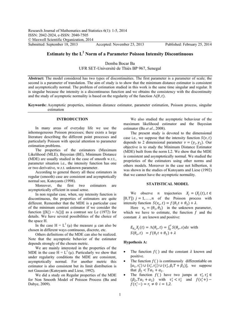
We observe 𝑛𝑛 trajectories 𝑋𝑋𝑗𝑗 = (𝑋𝑋𝑗𝑗 (𝑡𝑡), 𝑡𝑡 ∈
[0, 𝑇𝑇]) 𝑗𝑗 = 1, . . . , 𝑛𝑛 of the Poisson process with
intensity function 𝑆𝑆(𝜈𝜈𝑜𝑜 , 𝑡𝑡) = 𝑓𝑓(𝜃𝜃1 𝑡𝑡 + 𝜃𝜃2 ) + 𝜆𝜆.
Here 𝜈𝜈𝑜𝑜 = (𝜃𝜃1 , 𝜃𝜃2 ) in the unknown parameter,
which we have to estimate, the function 𝑓𝑓 and the
constant 𝜆𝜆 are known and positive:
𝑡𝑡
𝐸𝐸𝜃𝜃𝑜𝑜 𝑋𝑋𝑗𝑗 (𝑡𝑡) = Λ(𝜃𝜃𝑜𝑜 , 𝑡𝑡) = ∫0 𝑆𝑆(𝜃𝜃𝑜𝑜 , 𝑠𝑠)𝑑𝑑𝑑𝑑 with
𝑆𝑆(𝜃𝜃𝑜𝑜 , 𝑡𝑡) = 𝑓𝑓(𝜃𝜃1 𝑡𝑡 + 𝜃𝜃2 ) + 𝜆𝜆
Hypothesis A:
•
•
•
1
The function 𝑓𝑓( ) and the constant 𝜆𝜆 known and
positive.
The function 𝑓𝑓( ) is continuously differentiable on
[𝑎𝑎1 , 𝜏𝜏1∗ ) ∪ (𝜏𝜏1∗ , 𝜏𝜏2∗ ) ∪ (𝜏𝜏2∗ , 𝛽𝛽1 𝑇𝑇 + 𝛽𝛽2 )], we suppose
that 𝛽𝛽2 < 𝑇𝑇𝛼𝛼1 + 𝛼𝛼2 .
The function 𝑓𝑓( ) have two jumps at 𝜏𝜏1∗ , 𝜏𝜏2∗ ∈
(𝛽𝛽2 , 𝑇𝑇𝛼𝛼1 + 𝛼𝛼2 ) with 𝜏𝜏1∗ < 𝜏𝜏2∗ and 𝑓𝑓(𝜏𝜏𝑖𝑖∗ +) −
𝑓𝑓(𝜏𝜏𝑖𝑖∗ −) = 𝑟𝑟𝑖𝑖 ≠ 0 𝑖𝑖 = 1,2.
Res. J. Math. Stat., 6(1): 1-5, 2014
This leads to 𝜃𝜃1 = 𝜃𝜃 ′1 et 𝜃𝜃2 = 𝜃𝜃 ′ 2 i.e., 𝜃𝜃𝑜𝑜 = 𝜃𝜃 ′ 𝑜𝑜
which contradicts the fact that 𝜃𝜃𝑜𝑜 ≠ 𝜃𝜃 ′ 𝑜𝑜 .
So the lemma is proved.
We define this below the minimum distance
estimator of 𝜃𝜃𝑜𝑜 and we are intereste to their properties
when 𝑛𝑛 ⟶ ∞.
Let
𝐿𝐿2 ([0, 𝑇𝑇]) the Hilbert space with the
𝑇𝑇
Demonstration of the theorem: We put 𝑌𝑌𝑛𝑛 (𝑡𝑡) =
1 𝑛𝑛
∑ 𝑋𝑋 (𝑡𝑡) and 𝑍𝑍𝑛𝑛 (𝑡𝑡) = √𝑛𝑛 (𝑌𝑌𝑛𝑛 (𝑡𝑡) − Λ(𝜃𝜃𝑜𝑜 , 𝑡𝑡))which
𝑛𝑛 𝑗𝑗 =1 𝑗𝑗
allows to write for all 𝛿𝛿 > 0:
1/2
||ℎ( )|| = �∫0 ℎ2 (𝑡𝑡)� , then we define the minimum
distance estimator as solution of the equation:
1
1
�� ∑𝑛𝑛𝑗𝑗=1 𝑋𝑋𝑗𝑗 − Λ(𝜃𝜃𝑛𝑛∗ ,⋅)�� = 𝑖𝑖𝑖𝑖𝑖𝑖 �� ∑𝑛𝑛𝑗𝑗=1 𝑋𝑋𝑗𝑗 − Λ(𝜃𝜃,⋅)� |
𝑛𝑛
(𝑛𝑛)
STUDY OF THE CONSISTENCY
|𝜃𝜃 −𝜃𝜃𝑜𝑜 |≤𝛿𝛿
(𝑛𝑛)
The following theorem ensures the consistency of
the MDE.
≤ 𝑃𝑃𝜃𝜃𝑜𝑜 �2||𝑍𝑍𝑛𝑛 ( )|| > √𝑛𝑛𝜓𝜓(𝛿𝛿, 𝜃𝜃𝑜𝑜 )�
where, we have used the properties of the norm:
Theorem 1: If the Hypothesis 𝐴𝐴 is satisfied, then the
estimator of the minimum distance 𝜃𝜃𝑛𝑛∗ is consistent: for
all 𝛿𝛿 > 0:
𝑃𝑃𝜃𝜃 (𝑛𝑛 ) {𝜃𝜃𝑛𝑛∗ − 𝜃𝜃𝑜𝑜 | > 𝛿𝛿} ≤ 4
𝑜𝑜
𝑇𝑇
∫0 𝛬𝛬(𝜃𝜃𝑜𝑜 ,𝑡𝑡)𝑑𝑑𝑑𝑑
𝑛𝑛 𝜓𝜓(𝛿𝛿,𝜃𝜃𝑜𝑜 )2
�|𝑌𝑌𝑛𝑛 ( ) − Λ(𝜃𝜃𝑜𝑜 )|� + �|Λ(𝜃𝜃𝑜𝑜 ,⋅) − Λ(𝜃𝜃, )|�
≥ ||𝑌𝑌𝑛𝑛 ( ) − Λ(𝜃𝜃,⋅)||
||𝑌𝑌𝑛𝑛 ( ) − Λ(𝜃𝜃𝑜𝑜 , )|| − ||Λ(𝜃𝜃𝑜𝑜 ,⋅)|| ≤ ||𝑌𝑌𝑛𝑛 ( ) − Λ(𝜃𝜃,⋅)||
⟶0
Using the lemma 𝜓𝜓(𝛿𝛿, 𝜃𝜃𝑜𝑜 ) > 0. so, applying the
inequality of Chebychev it follows:
with 𝜓𝜓(𝛿𝛿, 𝜃𝜃𝑜𝑜 ) = inf|𝜃𝜃−𝜃𝜃𝑜𝑜 |>𝛿𝛿 ||Λ(𝜃𝜃,⋅) − Λ(𝜃𝜃𝑜𝑜 ,⋅)||
(𝑛𝑛)
For the demonstration of this theorem, we need the
following lemme.
𝑃𝑃𝜃𝜃 {2||𝑍𝑍𝑛𝑛 ( )||√𝑛𝑛 𝜓𝜓(𝛿𝛿, 𝜃𝜃𝑜𝑜 ) ≤
Because,
Lemme: If the Hypothesis 𝐴𝐴 is satisfied, then for all
𝛿𝛿 > 0, the function 𝜓𝜓(𝛿𝛿, 𝜃𝜃𝑜𝑜 ) > 0.
𝑇𝑇
𝑇𝑇
1
√𝑛𝑛
⟶0
2
∑𝑛𝑛1 ( 𝑌𝑌𝑗𝑗 (𝑡𝑡) − Λ(𝜃𝜃𝑜𝑜 , 𝑡𝑡)� 𝑑𝑑𝑑𝑑
= ∫0 ( Λ(𝜃𝜃𝑜𝑜 , 𝑡𝑡)𝑑𝑑𝑑𝑑
The latter term being bounded, which demonstrated
the theorem.
Asymptotic normality: In this section we will to prove
the Asymptotic Normality of MDE.
We define the functions 𝐹𝐹(𝜃𝜃, 𝑡𝑡) et 𝐺𝐺(𝜃𝜃, 𝑡𝑡) for all
𝑡𝑡 ∈ [0, 𝑇𝑇] as:
Λ(𝜃𝜃 ′ 𝑜𝑜 , 𝑡𝑡) = Λ(𝜃𝜃𝑜𝑜 , 𝑡𝑡)
since Λ(𝜃𝜃, 𝑡𝑡) is continuous function in 𝑡𝑡.
𝜕𝜕
𝜕𝜕
We deduce that Λ(𝜃𝜃 ′ 𝑜𝑜 , 𝑡𝑡) = Λ(𝜃𝜃𝑜𝑜 , 𝑡𝑡) for all
𝜕𝜕𝜕𝜕
𝜕𝜕𝜕𝜕
𝑡𝑡 ∈ [0, 𝑇𝑇] i.e.:
𝐹𝐹(𝜃𝜃, 𝑡𝑡) = −
𝜃𝜃2)
= 𝑓𝑓(𝜃𝜃 ′1 𝑡𝑡 + 𝜃𝜃 ′ 2 ) + 𝜆𝜆
= 𝑓𝑓(𝜃𝜃 ′1 𝑡𝑡 + 𝜃𝜃 ′ 2 )
1
𝜃𝜃1
𝑇𝑇
�∫0 𝑔𝑔 (𝜃𝜃1 𝑠𝑠 + 𝜃𝜃2 )𝑑𝑑𝑑𝑑 − 𝑡𝑡 𝑔𝑔(𝜃𝜃1 𝑡𝑡 +
et 𝐺𝐺(𝜃𝜃, 𝑡𝑡) = 𝑔𝑔(𝜃𝜃1 𝑡𝑡 + 𝜃𝜃2 ) − 𝑔𝑔(𝜃𝜃2 )
Let us notice that the functions 𝑅𝑅(𝜃𝜃, 𝑡𝑡) et 𝐺𝐺(𝜃𝜃, 𝑡𝑡)
are respectively the partial derives formal of the
function Λ(𝜃𝜃, 𝑡𝑡).
𝑇𝑇
Let us put 𝐴𝐴1,1 (𝜃𝜃) = ∫0 𝐹𝐹(𝜃𝜃, 𝑡𝑡)2 𝑑𝑑𝑑𝑑:
𝜃𝜃1 𝑡𝑡𝑠𝑠1 + 𝜃𝜃1 = 𝑟𝑟1 𝜃𝜃1 𝑡𝑡𝑠𝑠2 + 𝜃𝜃2 = 𝑟𝑟2
we have:
𝑡𝑡𝑠𝑠
� 1
𝑡𝑡𝑠𝑠2
𝑇𝑇
= ∫0 𝐸𝐸𝜃𝜃𝑜𝑜 �
so for all 𝑡𝑡 ∈ [0, 𝑇𝑇]:
𝑟𝑟1
𝜃𝜃
1
� � 1 � = �𝑟𝑟 �
1
𝜃𝜃2
2
𝑛𝑛𝑛𝑛 (𝛿𝛿,𝜃𝜃𝑜𝑜 )2
∫0 𝐸𝐸𝜃𝜃𝑜𝑜 (√𝑛𝑛(𝑌𝑌𝑛𝑛 (𝑡𝑡) − Λ(𝜃𝜃𝑜𝑜 , 𝑡𝑡)))2 𝑑𝑑𝑑𝑑
𝑖𝑖𝑖𝑖𝑖𝑖 ||Λ(𝜃𝜃,⋅) − Λ(𝜃𝜃𝑜𝑜 )|| = ||Λ(𝜃𝜃 ′ 𝑜𝑜 ) − Λ(𝜃𝜃𝑜𝑜 )|| = 0
with means that:
4𝐸𝐸𝜃𝜃 𝑜𝑜 ||𝑍𝑍𝑛𝑛 ( )||2
𝐸𝐸𝜃𝜃𝑜𝑜 ||𝑍𝑍𝑛𝑛 ( )||2
Demonstration: To show 𝜓𝜓(𝛿𝛿, 𝜃𝜃𝑜𝑜 ) > 0, proceed by
contradiction i.e., we suppose that for a 𝛿𝛿 > 0, we have
𝜓𝜓(𝛿𝛿, 𝜃𝜃𝑜𝑜 ) = 0.
In this case, it exist 𝜃𝜃𝑜𝑜 ≠ 𝜃𝜃 ′ 𝑜𝑜 such:
𝑓𝑓(𝜃𝜃1 𝑡𝑡 + 𝜃𝜃2 ) + 𝜆𝜆
𝑓𝑓(𝜃𝜃1 𝑡𝑡 + 𝜃𝜃2 )
(𝑛𝑛)
𝑃𝑃𝜃𝜃𝑜𝑜 ��|𝜃𝜃𝑛𝑛∗ − 𝜃𝜃𝑜𝑜 |� > 𝛿𝛿� ≤ 𝑃𝑃𝜃𝜃𝑜𝑜
inf �|𝑌𝑌𝑛𝑛 ( )– Λ(𝜃𝜃,⋅)|� >
|𝜃𝜃−𝜃𝜃𝑜𝑜 |≤𝛿𝛿
�
�
inf �|𝑌𝑌𝑛𝑛 ( )– Λ(𝜃𝜃, )|�
𝑛𝑛
𝑇𝑇
Λ2,2 (𝜃𝜃) = ∫0 𝐺𝐺(𝜃𝜃, 𝑡𝑡)2 𝑑𝑑𝑑𝑑
2
𝐴𝐴12
𝑇𝑇
= 𝐴𝐴2,1 = ∫0 𝐹𝐹 (𝜃𝜃, 𝑡𝑡) 𝐺𝐺(𝜃𝜃, 𝑡𝑡)𝑑𝑑𝑑𝑑
Res. J. Math. Stat., 6(1): 1-5, 2014
𝜕𝜕
2
𝐻𝐻 (𝜃𝜃) =
𝜕𝜕𝜃𝜃1 𝑛𝑛
𝜃𝜃1
𝑇𝑇
𝑡𝑡
∫0 �∫0 𝑔𝑔 (𝜃𝜃1 𝑠𝑠 +
1
� ∑𝑛𝑛𝑗𝑗=1 𝑋𝑋𝑗𝑗 (𝑡𝑡) −
𝑛𝑛
and
𝑇𝑇
𝑇𝑇
𝐶𝐶11 (𝜃𝜃) = ∫0 ∫0 𝐹𝐹 (𝜃𝜃, 𝑡𝑡)𝐹𝐹(𝜃𝜃, 𝑠𝑠)Λ(𝜃𝜃, 𝑠𝑠 ∧ 𝑡𝑡) 𝑑𝑑𝑑𝑑𝑑𝑑𝑑𝑑
𝐶𝐶2,2 (𝜃𝜃) =
𝐶𝐶1,2 (𝜃𝜃) =
𝑇𝑇 𝑇𝑇
∫0 ∫0 𝐺𝐺 (𝜃𝜃, 𝑡𝑡)𝐺𝐺(𝜃𝜃, 𝑠𝑠)Λ(𝜃𝜃, 𝑠𝑠 ∧ 𝑡𝑡) 𝑑𝑑𝑑𝑑𝑑𝑑𝑑𝑑
𝑇𝑇
𝑇𝑇
(𝜃𝜃, 𝑡𝑡)𝐺𝐺(𝜃𝜃, 𝑠𝑠)Λ(𝜃𝜃, 𝑠𝑠
𝐶𝐶2,1 (𝜃𝜃) = ∫0 ∫0 𝐹𝐹
Let be carrees matrix of order 2:
and
𝑑𝑑𝑑𝑑𝑑𝑑𝑑𝑑
∧ 𝑡𝑡)
𝜕𝜕
𝐻𝐻 (𝜃𝜃) =
𝜕𝜕𝜃𝜃2 𝑛𝑛
2 𝑇𝑇
− ∫0 [ 𝑔𝑔(𝜃𝜃1 𝑡𝑡
𝜃𝜃1
Λ(𝑡𝑡ℎ𝑒𝑒𝑡𝑡𝑎𝑎,𝑡𝑡 𝑑𝑑𝑡𝑡
𝐴𝐴11 (𝜃𝜃) 𝐴𝐴1,2 (𝜃𝜃)
�
𝐴𝐴(𝜃𝜃) = �
𝐴𝐴1,1 (𝜃𝜃) 𝐴𝐴2,1 (𝜃𝜃)
𝑇𝑇
1
𝑇𝑇
∗
∗
∗
𝑡𝑡 + 𝜃𝜃2,𝑛𝑛
) − 𝑔𝑔(𝜃𝜃2,𝑛𝑛
)�
∫0 �𝑔𝑔(𝜃𝜃1,𝑛𝑛
1
� ∑𝑛𝑛𝑗𝑗=1 𝑋𝑋𝑗𝑗 (𝑡𝑡) − Λ(𝜃𝜃𝑛𝑛∗ , 𝑡𝑡)� 𝑑𝑑𝑑𝑑 = 0
𝑛𝑛
−
We can write this system as:
Hypothesis B:
Théorème 2: If the Hypothesis 𝐴𝐴 and 𝐵𝐵 are satisfied
then the minimum distance estimator is asymptotically
normal i.e.:
−1
− 𝜃𝜃𝑜𝑜 ) ⟹ 𝑁𝑁(0, 𝒜𝒜 𝐶𝐶(𝜃𝜃𝑜𝑜 )𝒜𝒜 (𝜃𝜃𝑜𝑜 ))
thus,
𝑇𝑇
− Λ(𝜃𝜃, 𝑡𝑡)� 𝑑𝑑𝑑𝑑
𝜕𝜕
𝑇𝑇
𝑇𝑇
= √𝑛𝑛 ∫0 𝐺𝐺(𝜃𝜃𝑛𝑛∗ , 𝑡𝑡)[Λ(𝜃𝜃𝑛𝑛∗ , 𝑡𝑡) − Λ(𝜃𝜃𝑜𝑜 , 𝑡𝑡) 𝑑𝑑𝑑𝑑
Then,
𝑇𝑇
∫0 [ Λ(𝜃𝜃 + ℎ, 𝑡𝑡) − Λ(𝜃𝜃, 𝑡𝑡) − (ℎ, Λ(𝜃𝜃, 𝑡𝑡)
−(ℎ, Λ̇ (𝜃𝜃, 𝑡𝑡)2 𝑑𝑑𝑑𝑑 = 𝜃𝜃(|ℎ|2 )
Using the continuity of this functions and the
consistency of the estimator, we can write the system
as:
𝐻𝐻𝑛𝑛 (𝜃𝜃)𝜃𝜃=𝜃𝜃2 = 0
The calculation of the partial derives by report at
𝜃𝜃1 and 𝜃𝜃2 gives us:
𝑇𝑇
∫0 𝑊𝑊𝑛𝑛 (𝑡𝑡)𝐺𝐺(𝜃𝜃𝑛𝑛∗ , 𝑡𝑡) 𝑑𝑑𝑑𝑑
𝜃𝜃= Θ
𝜕𝜕𝜕𝜕
∑𝑛𝑛𝑗𝑗=1( 𝑋𝑋𝑗𝑗 (𝑡𝑡) − Λ(𝜃𝜃𝑜𝑜 , 𝑡𝑡))
= √𝑛𝑛 ∫0 𝐹𝐹(𝜃𝜃𝑛𝑛∗ , 𝑡𝑡)[Λ(𝜃𝜃𝑛𝑛∗ , 𝑡𝑡) − Λ(𝜃𝜃𝑜𝑜 , 𝑡𝑡) 𝑑𝑑𝑑𝑑
= 𝑎𝑎𝑎𝑎𝑎𝑎 inf 𝐻𝐻𝑛𝑛 (𝜃𝜃)
𝐻𝐻𝑛𝑛 (𝜃𝜃)𝜃𝜃 =𝜃𝜃1 = 0
1
√𝑛𝑛
∫0 𝑊𝑊𝑛𝑛 (𝑡𝑡)𝐹𝐹(𝜃𝜃𝑛𝑛∗ , 𝑡𝑡) 𝑑𝑑𝑑𝑑
2
∗
∗
, 𝜃𝜃2,𝑛𝑛
) and 𝜃𝜃 = (𝜃𝜃1 , 𝜃𝜃2 )
Let us note that 𝜃𝜃𝑛𝑛∗ = (𝜃𝜃1,𝑛𝑛
the function 𝐻𝐻𝑛𝑛 (𝜃𝜃) is derivable.
So the MDE 𝜃𝜃𝑛𝑛∗ minimize the function 𝐻𝐻𝑛𝑛 (𝜃𝜃) and
is consistent in 𝜃𝜃𝑜𝑜 element of Θ.
It with a probability numeric.
This estimator is a solution of system:
𝜕𝜕
1
𝑊𝑊𝑛𝑛 (𝑡𝑡) =
Let us remind that the minimum distance estimator
𝜃𝜃𝑛𝑛∗ is a solution of the equation:
𝜕𝜕𝜕𝜕
𝑇𝑇
We introduce the process us 𝑊𝑊𝑛𝑛 () define by:
Demonstration: We define the function 𝐻𝐻𝑛𝑛 (𝜃𝜃) by:
𝜃𝜃𝑛𝑛∗
1
∫0 𝐺𝐺 (𝜃𝜃𝑛𝑛∗ , 𝑡𝑡) �𝑛𝑛 ∑𝑛𝑛𝑗𝑗=1 𝑋𝑋𝑗𝑗 (𝑡𝑡) − Λ(𝜃𝜃𝑜𝑜 , 𝑡𝑡) + Λ(𝜃𝜃𝑜𝑜 , 𝑡𝑡) −
Λ(𝜃𝜃𝑛𝑛∗,𝑡𝑡)𝑑𝑑𝑡𝑡=0
𝐴𝐴11 (𝜃𝜃) 𝐴𝐴2,2 (𝜃𝜃) ≠ (𝐴𝐴1,2 (𝜃𝜃))2
𝐻𝐻𝑛𝑛 (𝜃𝜃) =
𝑇𝑇
∫0 𝐹𝐹 (𝜃𝜃𝑛𝑛∗ , 𝑡𝑡) �𝑛𝑛 ∑𝑛𝑛𝑗𝑗=1 𝑋𝑋𝑗𝑗 (𝑡𝑡) − Λ(𝜃𝜃𝑜𝑜 , 𝑡𝑡) + Λ(𝜃𝜃𝑜𝑜 , 𝑡𝑡) −
Λ(𝜃𝜃𝑛𝑛∗,𝑡𝑡)𝑑𝑑𝑡𝑡=0
To prove the asymptotic normality, we suppose that:
∑𝑛𝑛𝑗𝑗=1 𝑋𝑋𝑗𝑗 (𝑡𝑡)
𝑡𝑡
𝑛𝑛
𝑇𝑇
�∫0 𝐹𝐹 (𝜃𝜃, 𝑡𝑡)𝐺𝐺(𝜃𝜃, 𝑡𝑡)𝑑𝑑𝑑𝑑�
𝑇𝑇 1
∫0 �𝑛𝑛
𝑛𝑛
� ∑𝑛𝑛𝑗𝑗=1 𝑋𝑋𝑗𝑗 (𝑡𝑡) − Λ(𝜃𝜃𝑛𝑛∗ , 𝑡𝑡)� 𝑑𝑑𝑑𝑑 = 0
𝑇𝑇
𝑇𝑇
∫0 𝐹𝐹 (𝜃𝜃, 𝑡𝑡)2 𝑑𝑑𝑑𝑑 ∫0 𝐺𝐺 (𝜃𝜃, 𝑡𝑡)2 𝑑𝑑𝑑𝑑
2
−1
1
+ 𝜃𝜃2 − 𝑔𝑔(𝜃𝜃2 )] � ∑𝑛𝑛𝑗𝑗=1 𝑋𝑋𝑗𝑗 (𝑡𝑡) −
∗
∗
∗
∗
𝑠𝑠 + 𝜃𝜃2,𝑛𝑛
)𝑑𝑑𝑑𝑑 − 𝑡𝑡𝑡𝑡(𝜃𝜃1,𝑛𝑛
𝑡𝑡 + 𝜃𝜃2,𝑛𝑛
)�
∫0 �∫0 𝑔𝑔 (𝜃𝜃1,𝑛𝑛
the determinant of the matrix 𝐴𝐴(𝜃𝜃) is:
√𝑛𝑛(𝜃𝜃𝑛𝑛∗
Λ(𝜃𝜃, 𝑡𝑡)� 𝑑𝑑𝑑𝑑
thus using (3) and (4), we obtain:
𝐶𝐶 (𝜃𝜃) 𝐶𝐶12 (𝜃𝜃)
𝐶𝐶(𝜃𝜃) = � 11
�
𝐶𝐶21 (𝜃𝜃) 𝐶𝐶2,2 (𝜃𝜃)
𝑑𝑑e𝑡𝑡(𝐴𝐴(𝜃𝜃)) =
𝜃𝜃2 )𝑑𝑑𝑑𝑑 − 𝑡𝑡𝑡𝑡(𝜃𝜃1 𝑡𝑡 + 𝜃𝜃2 )� ×
𝑇𝑇
3
∫0 𝑊𝑊𝑛𝑛 (𝑡𝑡)𝐹𝐹(𝜃𝜃𝑜𝑜 , 𝑡𝑡)𝑑𝑑𝑑𝑑
𝑇𝑇
= ∫ 𝐹𝐹(𝜃𝜃𝑜𝑜 , 𝑡𝑡)(𝑢𝑢𝑛𝑛∗ , Λ̇ (𝜃𝜃𝑜𝑜 , 𝑡𝑡)𝑑𝑑𝑑𝑑 + 𝜃𝜃(1)
0
Res. J. Math. Stat., 6(1): 1-5, 2014
𝑇𝑇
𝐶𝐶ℓ,𝑖𝑖 (𝜃𝜃𝑜𝑜 ) = 𝐸𝐸𝜃𝜃𝑜𝑜 (𝑌𝑌 (ℓ) 𝑌𝑌 (𝑖𝑖) )
∫0 𝑊𝑊𝑛𝑛 (𝑡𝑡)𝐺𝐺(𝜃𝜃𝑜𝑜 , 𝑡𝑡)𝑑𝑑𝑑𝑑
𝑇𝑇
= ∫ 𝐺𝐺(𝜃𝜃𝑜𝑜 , 𝑡𝑡)(𝑢𝑢𝑛𝑛∗ , Λ̇ (𝜃𝜃𝑜𝑜 , 𝑡𝑡)) 𝑑𝑑𝑑𝑑 + 𝜃𝜃(1)
0
We obtain:
∗
∗
where we put 𝑢𝑢𝑛𝑛∗ = (𝑢𝑢1𝑛𝑛
, 𝑢𝑢∗ 2𝑛𝑛)𝑡𝑡 , 𝑢𝑢1,𝑛𝑛
= √𝑛𝑛(𝜃𝜃 ∗ 1, 𝑛𝑛 −
∗
∗
𝜃𝜃1 ) et 𝑢𝑢2,𝑛𝑛 = (√𝑛𝑛(𝜃𝜃2,𝑛𝑛 − 𝜃𝜃2 ) we introduce the vector
(1)
(2)
𝑌𝑌𝑛𝑛 = (𝑌𝑌𝑛𝑛 , 𝑌𝑌𝑛𝑛 )𝑇𝑇
with,
(1)
𝑌𝑌𝑛𝑛
(2)
𝑌𝑌𝑛𝑛
(1)
𝑌𝑌𝑛𝑛
(2)
𝑌𝑌𝑛𝑛
and,
𝑇𝑇
= ∫0 𝐹𝐹 (𝜃𝜃𝑜𝑜 , 𝑡𝑡) 𝑊𝑊𝑛𝑛 (𝑡𝑡) 𝑑𝑑𝑑𝑑
𝑇𝑇
𝑇𝑇
1
=
=
𝑇𝑇
∑𝑛𝑛𝑗𝑗=1( 𝑋𝑋𝑗𝑗 (𝑡𝑡) − Λ(𝜃𝜃𝑜𝑜 , 𝑡𝑡)� 𝐹𝐹(𝜃𝜃𝑜𝑜 , 𝑡𝑡) 𝑑𝑑𝑑𝑑
we obtain for example:
𝑇𝑇
(1)
𝑠𝑠𝑑𝑑𝑠𝑠 𝑑𝑑𝑡𝑡
1
√𝑛𝑛
1
√𝑛𝑛
as √𝑛𝑛(𝜃𝜃𝑛𝑛∗ − 𝜃𝜃𝑜𝑜 ) = 𝐵𝐵(𝜃𝜃𝑜𝑜 ) 𝑌𝑌𝑛𝑛 + 𝜃𝜃(1)
𝑇𝑇
∑𝑛𝑛𝑗𝑗=1 ∫0 ( 𝑋𝑋𝑗𝑗 (𝑡𝑡) − Λ(𝜃𝜃𝑜𝑜 , 𝑡𝑡)𝐺𝐺(𝜃𝜃𝑜𝑜 , 𝑡𝑡)𝑑𝑑𝑑𝑑
we deduce:
𝑢𝑢𝑛𝑛∗ = √𝑛𝑛(𝜃𝜃𝑛𝑛∗ − 𝜃𝜃𝑜𝑜 ) ⟹ 𝒩𝒩(0, 𝐵𝐵(𝜃𝜃𝑜𝑜 ) 𝐶𝐶(𝜃𝜃𝑜𝑜 ) 𝐵𝐵(𝜃𝜃𝑜𝑜 )𝑡𝑡 ) i.e.:
√𝑛𝑛(𝜃𝜃𝑛𝑛∗ − 𝜃𝜃𝑜𝑜 ) ⟹ 𝒩𝒩(0, 𝐴𝐴−1 (𝜃𝜃𝑜𝑜 ) 𝐶𝐶(𝜃𝜃𝑜𝑜 ) 𝐴𝐴−1 (𝜃𝜃𝑜𝑜 )𝑡𝑡 )
Let us note that the terms of the matrix are:
𝑇𝑇
So the asymptotic normality is proved.
𝑇𝑇
𝑌𝑌 (1) = ∫0 �∫𝑡𝑡 𝐹𝐹(𝜃𝜃𝑜𝑜 , 𝑠𝑠) 𝑑𝑑𝑑𝑑� 𝑑𝑑𝑑𝑑(Λ(𝜃𝜃𝑜𝑜 , 𝑡𝑡))
𝑌𝑌 (2) =
𝑇𝑇
𝑇𝑇
∫0 �∫𝑡𝑡 𝐺𝐺(𝜃𝜃𝑜𝑜 , 𝑠𝑠)𝑑𝑑𝑑𝑑�
We have the following relation:
𝑇𝑇
𝑌𝑌𝑛𝑛 ⟹ 𝒩𝒩(0, 𝐶𝐶(𝜃𝜃𝑜𝑜 ))
∑𝑛𝑛𝑗𝑗=1 𝜓𝜓𝑗𝑗(2) with 𝜓𝜓𝑗𝑗(1)
√𝑛𝑛
𝑇𝑇
= ∫0 ( 𝑋𝑋𝑗𝑗 (𝑡𝑡) − Λ(𝜃𝜃𝑜𝑜 , 𝑡𝑡))𝐺𝐺(𝜃𝜃𝑜𝑜 , 𝑡𝑡)𝑑𝑑𝑑𝑑
(1) (2)
𝐸𝐸𝜃𝜃𝑜𝑜 𝜓𝜓𝑗𝑗 𝜓𝜓𝑗𝑗 = 𝐶𝐶ℓ,𝑖𝑖 (𝜃𝜃𝑜𝑜 )
=
𝑇𝑇
= ∫0 ∫0 𝐹𝐹(𝜃𝜃𝑜𝑜 , 𝑡𝑡)𝐺𝐺(𝜃𝜃𝑜𝑜 , 𝑠𝑠)Λ(𝜃𝜃𝑜𝑜 , 𝑡𝑡 ∧
Using the central theorem limit, we obtain:
= ∫0 � ) ∑𝑛𝑛𝑗𝑗=1( 𝑋𝑋𝑗𝑗 (𝑡𝑡) − Λ(𝜃𝜃𝑜𝑜 , 𝑡𝑡)� 𝐹𝐹(𝜃𝜃𝑜𝑜 , 𝑡𝑡) 𝑑𝑑𝑑𝑑
=
(2)
𝐸𝐸𝜃𝜃𝑜𝑜 𝜓𝜓1 𝜓𝜓1
∫0 𝐺𝐺(𝜃𝜃𝑜𝑜 , 𝑡𝑡) 𝑊𝑊𝑛𝑛 (𝑡𝑡) 𝑑𝑑𝑑𝑑
1
𝑡𝑡
𝐸𝐸𝜃𝜃𝑜𝑜 [𝑋𝑋1 (𝑡𝑡) − Λ(𝜃𝜃𝑜𝑜 , 𝑡𝑡)][𝑋𝑋1 (𝑠𝑠) − Λ(𝜃𝜃𝑜𝑜 , 𝑠𝑠) =
Λ(𝜃𝜃𝑜𝑜 , 𝑡𝑡 ∧ 𝑠𝑠]
∑𝑛𝑛 𝜓𝜓 (1) with 𝜓𝜓𝑗𝑗(1)
√𝑛𝑛 𝑗𝑗 =1 𝑗𝑗
𝑇𝑇
∫0 ( 𝑋𝑋𝑗𝑗 (𝑡𝑡) − Λ(𝜃𝜃𝑜𝑜 , 𝑡𝑡))𝐹𝐹(𝜃𝜃𝑜𝑜 , 𝑡𝑡)𝑑𝑑𝑑𝑑
𝑇𝑇
𝑇𝑇
= ∫0 ∫𝑠𝑠 𝐺𝐺(𝜃𝜃𝑜𝑜 , 𝑡𝑡)𝑑𝑑𝑑𝑑 𝑑𝑑𝑑𝑑(𝑠𝑠)
On the other hand using:
∑𝑛𝑛𝑗𝑗=1 ∫0 ( 𝑋𝑋𝑗𝑗 (𝑡𝑡) − Λ(𝜃𝜃𝑜𝑜 , 𝑡𝑡)𝐹𝐹(𝜃𝜃𝑜𝑜 , 𝑡𝑡) 𝑑𝑑𝑑𝑑
1
𝑇𝑇
𝑇𝑇
= ∫0 ∫𝑠𝑠 𝐹𝐹(𝜃𝜃𝑜𝑜 , 𝑡𝑡) 𝑑𝑑𝑑𝑑𝑑𝑑𝑑𝑑(𝑠𝑠)
(2)
𝜓𝜓1
∫0 𝐹𝐹 (𝜃𝜃𝑜𝑜 , 𝑡𝑡)𝑊𝑊𝑛𝑛 (𝑡𝑡)𝑑𝑑𝑑𝑑
√𝑛𝑛
𝑇𝑇
𝑇𝑇
(2)
We show that 𝑛𝑛 𝐸𝐸𝜃𝜃𝑜𝑜 (𝜃𝜃𝑛𝑛∗ − 𝜃𝜃𝑜𝑜 )(𝜃𝜃𝑛𝑛∗ − 𝜃𝜃𝑜𝑜 )𝑡𝑡 =
𝐵𝐵(𝜃𝜃𝑜𝑜 )𝐶𝐶(𝜃𝜃𝑜𝑜 ) 𝐵𝐵(𝜃𝜃𝑜𝑜 )𝑡𝑡 + 𝜃𝜃(1)
We have:
1
𝑇𝑇
For 𝜓𝜓1 we have:
𝑢𝑢𝑛𝑛∗ = 𝐵𝐵(𝜃𝜃𝑜𝑜 )𝑌𝑌𝑛𝑛 + 𝜃𝜃(1)
√𝑛𝑛
𝑇𝑇
= ∫0 ∫𝑠𝑠 10≤𝑠𝑠≤𝑡𝑡 [𝑑𝑑𝑋𝑋1 (𝑠𝑠) − 𝑆𝑆(𝜃𝜃𝑜𝑜 , 𝑡𝑡) 𝑑𝑑𝑑𝑑] 𝐹𝐹(𝜃𝜃𝑜𝑜 , 𝑡𝑡) 𝑑𝑑𝑑𝑑
= ∫0 ∫0 𝐹𝐹(𝜃𝜃𝑜𝑜 , 𝑡𝑡) 𝑑𝑑𝑑𝑑[𝑑𝑑𝑋𝑋1 (𝑠𝑠) − 𝑆𝑆(𝜃𝜃𝑜𝑜 , 𝑡𝑡) 𝑑𝑑𝑑𝑑]
From the hypothesis 𝐵𝐵, the matrix of order 2 𝐴𝐴(𝜃𝜃𝑜𝑜 )
is invertible thus we can write 𝐵𝐵(𝜃𝜃𝑜𝑜 ) = 𝐴𝐴(𝜃𝜃𝑜𝑜 )−1 , so:
𝑇𝑇
𝑇𝑇
= ∫0 [ 𝑋𝑋1 (𝑡𝑡) − Λ(𝜃𝜃𝑜𝑜 , 𝑡𝑡)] 𝐹𝐹(𝜃𝜃𝑜𝑜 , 𝑡𝑡) 𝑑𝑑𝑑𝑑
𝐴𝐴𝑛𝑛 (𝜃𝜃𝑜𝑜 ) 𝑢𝑢𝑛𝑛∗ = 𝑌𝑌𝑛𝑛 + 𝜃𝜃(1)
= ∫0 �
2
𝑇𝑇
𝑇𝑇
𝑇𝑇
(1)
𝜓𝜓1
or under matrix shape:
𝑇𝑇
𝑇𝑇
𝐶𝐶2,2 (𝜃𝜃𝑜𝑜 ) = ∫0 �∫𝑡𝑡 𝐺𝐺(𝜃𝜃𝑜𝑜 , 𝑠𝑠) 𝑑𝑑𝑑𝑑� 𝑆𝑆(𝜃𝜃𝑜𝑜 , 𝑡𝑡) 𝑑𝑑𝑑𝑑
∫0 �∫𝑡𝑡 𝐹𝐹(𝜃𝜃𝑜𝑜 , 𝑠𝑠) 𝑑𝑑𝑑𝑑 ∫0 𝐺𝐺 (𝜃𝜃𝑜𝑜 , 𝑟𝑟) 𝑑𝑑𝑑𝑑� 𝑆𝑆(𝜃𝜃𝑜𝑜 , 𝑡𝑡) 𝑑𝑑𝑑𝑑
∗
∗
𝐴𝐴1,1 (𝜃𝜃𝑜𝑜 )𝑢𝑢1,𝑛𝑛
) + 𝐴𝐴1,2 (𝜃𝜃𝑜𝑜 )𝑢𝑢2,𝑛𝑛
+ 𝜃𝜃(1)
∗
𝐴𝐴2,1 (𝜃𝜃𝑜𝑜 )𝑢𝑢1,𝑛𝑛 𝑡𝑡) + 𝐴𝐴2,2 (𝜃𝜃𝑜𝑜 ) + 𝜃𝜃(1)
=
2
𝑇𝑇
= ∫0 �∫𝑡𝑡 𝐹𝐹(𝜃𝜃𝑜𝑜 , 𝑠𝑠) 𝑑𝑑𝑑𝑑� 𝑆𝑆(𝜃𝜃𝑜𝑜 , 𝑡𝑡) 𝑑𝑑𝑑𝑑
𝐶𝐶1,2 (𝜃𝜃𝑜𝑜 ) = 𝐶𝐶2,1 (𝜃𝜃𝑜𝑜 ) =
= ∫0 𝐺𝐺 (𝜃𝜃𝑜𝑜 , 𝑡𝑡) 𝑊𝑊𝑛𝑛 (𝑡𝑡) 𝑑𝑑𝑑𝑑 we obtain
=
𝑇𝑇
𝐶𝐶1,1 (𝜃𝜃𝑜𝑜 )
REFERENCES
𝑑𝑑𝑑𝑑�Λ(𝜃𝜃𝑜𝑜 , 𝑡𝑡)�
Ba, D.B. and A.S. Dabye, 2009. On regular properties
of the MDE for non smooth model of poisson
process, Indian J. Math., 51(1): 145-162.
4
Res. J. Math. Stat., 6(1): 1-5, 2014
Ba, D.B., A.S. Dabye, A. Diakhaby and F.N. Diop,
2008. Comportment asymptotique des estimateurs
de paramètre d’un processus de Poisson pour un
modèle non régulier. Annales de l’Université
Ndjamena, 3: 55-65.
Kutoyants, Y.A., 1998. Statistical Inference for Spatial
Poisson Processes, Lect. Notes Statist. 134,
Springer, New York, pp: 276.
Kutoyants, Y.A. and F. Liese, 1992. On minimum
distance estimation for spatial poisson processes.
Ann. Academial. Scient. Fennicae, ser. A. I., 17:
65-71.
Le, C., 1972. Limit of experiments. Proceeding of the
6th Berkeley Symposium on Mathematical
Statistics and Probability,1: 245-261.
5