Modal Frequency Response Analysis using MSC.Nastran
advertisement
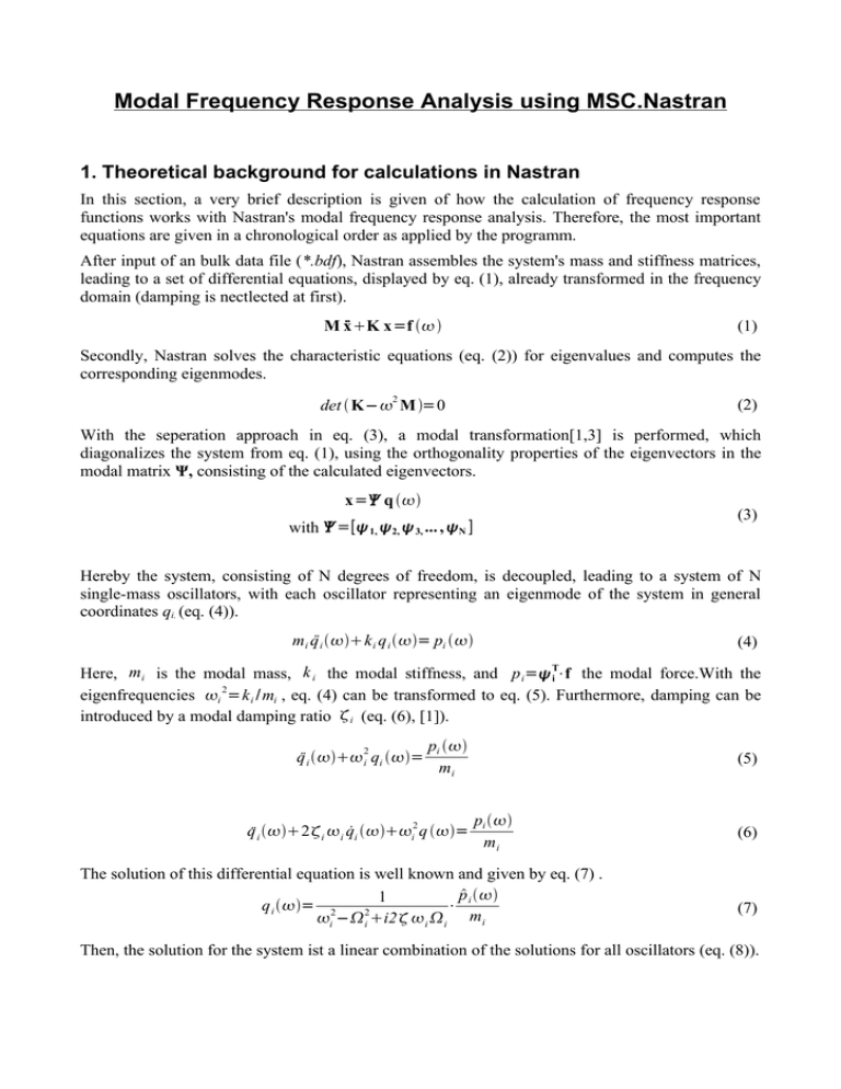
Modal Frequency Response Analysis using MSC.Nastran 1. Theoretical background for calculations in Nastran In this section, a very brief description is given of how the calculation of frequency response functions works with Nastran's modal frequency response analysis. Therefore, the most important equations are given in a chronological order as applied by the programm. After input of an bulk data file (*.bdf), Nastran assembles the system's mass and stiffness matrices, leading to a set of differential equations, displayed by eq. (1), already transformed in the frequency domain (damping is nectlected at first). M ẍK x=f (1) Secondly, Nastran solves the characteristic equations (eq. (2)) for eigenvalues and computes the corresponding eigenmodes. 2 (2) det K− M =0 With the seperation approach in eq. (3), a modal transformation[1,3] is performed, which diagonalizes the system from eq. (1), using the orthogonality properties of the eigenvectors in the modal matrix Ψ, consisting of the calculated eigenvectors. x= q (3) with =[ 1, 2, 3, ... , N ] Hereby the system, consisting of N degrees of freedom, is decoupled, leading to a system of N single-mass oscillators, with each oscillator representing an eigenmode of the system in general coordinates qi. (eq. (4)). mi q̈ i k i q i = pi (4) Here, mi is the modal mass, k i the modal stiffness, and p i= Ti ⋅f the modal force.With the eigenfrequencies i 2=k i /mi , eq. (4) can be transformed to eq. (5). Furthermore, damping can be introduced by a modal damping ratio i (eq. (6), [1]). q̈ i 2i qi = pi mi q̈ i 2i i q̇i i2 q = (5) pi mi The solution of this differential equation is well known and given by eq. (7) . p 1 q i = 2 ⋅ i 2 i −i i2 i i mi (6) (7) Then, the solution for the system ist a linear combination of the solutions for all oscillators (eq. (8)). N x =∑ i q i (8) i =1 The frequency response function is defined as the ratio of the response of a system x (displacement, velocity, acceleration) to its excitation force F . The FRF for displacement of the system is given by eq. (9). H = x N Ti 1 =∑ i⋅ 2 ⋅ F i=1 i − i2i2 i i mi (9) Thus, the FRF for the kth node (degree of freedom) with an single excitation force at jth dof can be calculated by eq. (10). N i k⋅ i j H k =∑ (10) 2 2 i=1 m i i −i i2 i i 2. Pre-processing with Patran In this case a simple model of a cantilever plate under a single-point cyclic load is used. In the preprocessing step the model geometry, the finite element mesh, the loads and boundary conditions and material properties have to be generated. Also, the load cases and the Nastran case controls parameters have to be defined. With these informations the Nastran bulk data file is automatically created by Patran created. A. Geometry: − Create a Surface: − length: 30mm − height: 10mm B. Elements: − Generate a regular isometric mesh: − globale edge-length: 1 mm − 10 x 30 elements C. Loads − In this example for one edge of the plate all six degrees of freedom are fixed. Further, a single point load with the magnitude 10 N is applied at a certain node. − 1. Generating boundary constraints: − 2. Generating force: D. Materials / Properties − 1. Define material properties: − Aluminum: E = 70.000 N/mm2 ρ = 2,7E-6 kg/mm3 υ = 0,3 − 2. Define model properties: − thickness: 2 mm E. Analysis − 1. Solution Type: − Frequency response analysis, modal formulation(SOL 111) − − Solution Parameters [2]: − Residual Vector Computation for decreasing modal truncation error − Coupled Mass calculation − Rz stiffness to prevent singularities in matrix Eigenvalue Extraction: − Lanczos algorithm − Frequency range: − − 0 – 4000 Hz undefined number of roots (eigenfrequencies) in range of interest 1. 2. 3. − 2. Subcases: − select the Default subcase a) − Subcase Parameters: − Define frequencies: table for frequency response analysis (5 Hz increments), this frequency table is used for generating the cyclic frequency of an harmonic excitation force, the amplitude is the prior defined singlepoint load − Crit. modal damping, define constant modal damping ratios via table (ς = 0,001 for all modes; values are extra/interpolated from table for each mode) a) b) b) − 3. Subcases Select: − − Select the Default subcase Run Analysis! 3. Post-processing with Patran A. Analysis − Access Results: − check correct Job Name − (Select Results File -> *.xdb) B. Results: − 1. Graph the FRF − Select Result Cases − Filter subcases − display Z-Component of displacement function over frequency − i.e. for the excitation node, with logarithmic scaling of y-axis, magnitude − − The resulting graph should look like this: − It is also possible to select the phase, real or imaginary part of the displacement function for display 2. Print the results in a file (for import in Excel or similar) − i.e. magnitude for excitation node 4. Damaged Model A simple damaged model can be created by deletion of several elements. This is examplary shown in this section A. Deletions of elements – Go back to Elements – select Action: Delete, Object: Element – select the desired element B. Analysis and Postprocessing – Perform analysis with the same parameters, but a different job name (i.e. exercise_dam) – Attach the new *.xdb-file – Go to Results – filter out the new subcases (filter method: subcase ids) – Make sure that the desired node ist selected. – Check the box for Append Curves in XY Window on the Display Attributes card. – All other parameters are the same. 5. Remarks − Natural frequencies can be extracted from *.f06-files − Possible variations of results: − Comparison of FRFs for different nodes − FRFs for accelerations, velocities can be calculated (Analysis -> Subcases -> Output requests -> Select ...) − Calculate Resonances (with damping influence...) from extracted data... − Given is the simplest case of excitation, more complicated excitation loads can be created using tables and fields (i.e. white noise excitation) 6. Literature [1] Da Silva, Clarence W. (1999). Vibration: Fundamentals and Practice. CRC Press LCC [2] MSC.Software Corporation (2003). MSC.Nastran 2004 - Release Guide. MSC.Software Corporation, Santa Ana, CA, USA. [3] Hörnlund, M. and Papazoglu, A. (2005). Analysis and measurements of vehicle door structural dynamic response. Divison of Structural Mechanics, Lund University, Sweden. http://www.byggmek.lth.se/fileadmin/byggnadsmekanik/ publications/tvsm5000/web5131.pdf 7. Appendix − MSC.Nastran Bulk Data File
