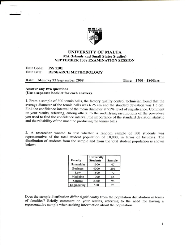
UNIVERSITY OF MALTA
MA (Islands and Small States Studies)
SEPTEMBER 2008 EXAMINATION SESSION
Unit Code:
Unit Title:
ISS 5101
RESEARCH METHODOLOGY
Time: 1700 - ISOOhrs
Date: Monday 22 September 2008
Answer any two questions
(Use a separate booklet for each answer).
1. From a sample of 300 tennis balls, the factory quality control technician found that the
average diameter of the tennis balls was 6.25 cm and the standard deviation was 1.5 cm.
Find the confidence interval of the mean diameter at 95% level of significance. Comment
on your results, referring, among others, to the underlying assumptions of the procedure
you used to find the confidence interval, the importance of the standard deviation statistic
and the reliability of the machine producing the tennis balls
2. A researcher wanted to test whether a random sample of 500 students was
representative of the total student population of 10,000, in terms of faculties. The
distribution of students from the sample and from the total student population is shown
below:
Faculty
Humanities
Business
Law
Medicine
Science
Engineering
University
Students
1000
4000
1500
1000
2000
500
Sample
47
206
72
56
96
23
Does the sample distribution differ significantly from the population distribution in terms
of faculties? Briefly comment on your results, referring to the need for having a
representative sample when seeking information about the population.
3. A researcher tried to find why some girls were more successful than others in their
occupation as salesgirls and carried out a multiple regression analysis towards this end,
using a sample size of 30 persons. He obtained the following results:
SLS -14.8 + 2.0 CLS - 1.0 EXP - 2.1 DST + 10.0 TCH
t-statistic
(1.5)
(8.1)
(-0.9)
(-2.1)
(2.5)
p-values
[0.15] [0.0]
[0.39]
[0.05]
[0.03]
R2 = 0.893
Where: SLS = sales in hundreds of dollars
CLS = number of sales calls per month
Exp — number of years experience
DST= mean driving distance to each call
TCH = A dummy variable taking the value of 0 = No, 1 = Yes and refers
to whether the sales person is using a new high-tech sales system.
The researcher also found that the correlation between the explanatory variables CLS,
DIS and TCH was in all cases lower than 0.4, whereas that between CLS and EXP was
rather hi ghat 0.8
Comment on the results referring to the causal relationships and the statistical
significance of the estimated coefficients. What can we predict from the results?
4. Answer both 4a and 4b.
4a. Describe briefly with an example the aim and use of the following procedures
within the SPSS package: the case summaries procedure, the replace missing values
procedure and the recode into different variables procedure.
and
4b. Explain the use of the histogram, the pie chart and the scatter plot provided in the
SPSS package. Discuss the main instances when such graphical methods are used and
the main information which can be derived from these graphical tools
5. Answer either 5a or 5b
5a. Distinguish between qualitative and quantitative research. Discuss some strengths
of qualitative research.
91
5b. Describe a procedure for conducting a survey in order to assess the attitudes of
adults residing in Malta regarding bus public transport.
Appendix IV
Percentile Values (xzp)
for
the Chi-Square Distribution
with v Degrees of Freedom
(shaded area — p )
V
1
x2
x2
6.63
X2
x2
2.71
4.61
6.25
7.78
1.32
2.77
4.11
5.39
.455
1.39
3
14.9
11.3
13.3
9.35
11.1
5
6
7
16.7
18.5
20.3
15.1
16.8
18.5
8
9
22.0
23.6
20.1
21.7
12.8
14.4
16.0
17.5
19.0
11.1
12.6
14.1
15.5
16.9
9.24
10.6
12.0
13.4
14.7
6.63
7.84
9.04
10.2
11.4
10
11
12
13
14
25.2
26.8
23.2
28.3
29.8
31.3
26.2
27.7
29.1
20.5
21.9
23.3
24.7
26.1
18.3
19.7
21.0
22.4
23.7
16.0
17.3
18.5
19.8
21.1
12.5
13.7
14.8
16.0
17.1
32.8
34.3
27.5
28.8
30.2
31.5
32.9
25.0
26.3
27.6
28.9
30.1
22.3
23.5
24.8
26.0
27.2
18.2
19.4
20.5
21.6
38.6
30.6
32.0
33.4
34.8
36.2
40.0
37.6
41.4
42.8
44.2
45.6
38.9
41.6
43.0
34.2
35.5
36.8
38.1
39.4
31.4
32.7
33.9
35.2
36.4
28.4
29.6
30.8
32.0
23.8
24.9
26.0
27.1
28.2
44.3
45.6
47.0
48.3
49.6
40.6
41.9
43.2
44.5
45.7
37.7
38.9
40.1
41.3
42.6
34.4
35.6
36.7
43.8
55.8
67.5
79.1
40.3
90.5
101.9
113.1
124.3
15
16
17
18
19
20
21
22
23
24
25
26
27
28
29
35.7
37.2
46.9
48.3
49.6
51.0
52.3
24.7
40.3
7.81
9.49
x
2
A.50
4
9.21
3.84
5.99
x
2
A.75
7.88
10.6
12.8
2
5.02
7.38
2
30
53.7
40
66.8
50
79.5
50.9
63.7
76.2
60
92.0
88.4
47.0
59.3
71.4
83.3
70
80
90
100
104.2
116.3
128.3
140.2
100.4
112.3
124.1
135.8
95.0
106.6
118.1
129.6
33.2
37.9
39.1
51.8
63.2
74.4
85.5
96.6
107.6
118.5
22.7
2.37
3.36
4.35
5.35
6.35
7.34
8.34
9.34
10.3
11.3
12.3
13.3
14.3
15.3
16.3
17.3
18.3
19.3
20.3
21.3
22.3
23.3
x
•\225
.102
.575
1.21
1.92
2.67
3.45
4.25
5.07
5-90
6.74
7.58
8.44
9.30
10.2
11.0
11.9
12.8
13.7
14.6
15.5
16.3
17,2
18.1
19.0
19,9
20.8
21.7
22.7
2
x2
.0158
.211
.584
1.06
1.61
2.20
2.83
3.49
4.17
4.87
5.58
6.30
7.04
7.79
8.55
9.31
10.1
10.9
11.7
12.4
13.2
14.0
14.8
15.7
.0039
.103
.352
.711
.831
1.24
1.69
2.18 .
2.70
.554
.872
1.24
1.65
2.09
3.94
4.57
5.23
5.89
6.57
3.25
3.82
4.40
5.01
5.63
2.56
3.05
3.57
4.11
4.66
7.26
7.96
8.67
9.39
10.1
6.26
6.91
7.56
8.23
8.91
5.23
5.81
6.41
7.01
7.63
10.9
11.6
12.3
13.1
13.8
9.59
10.3
11.0
11.7
8.26
8.90
9.54
10.2
7.43
12.4
10.9
9.89
13.1
13.8
11.5
12.2
14.6
15.3
16.0
12.9
13.6
14.3
12.5
16.8
24.4
32.4
15.0
22.2
29.7
13.8
20.7
28.0
40.5
37.5
35.5
48.8
57.2
65.6
45.4
53.5
61.8
43.3
51.2
74.2
70.1
24.5
33.7
42.9
52.3
20.6
29.1
37.7
46.5
18.5
26.5
67.0
29.3
39.3
49.3
59.3
77.6
88.1
98.6
109.1
69.3
79.3
89.3
99.3
61.7
71.1
80.6
90.1
55.3
64.3
73.3
34.8
45.6
56.3
82.4
.0000
.0100
.072
.207
1.15
1.64
2.17
2.73
3.33
23.6
26.3
27.3
28.3
.0010 .0002
.0506 .0201
.216 .115
.297
14.6
15.4
16.2
16.9
24.3
25.3
X.005
2
Y2
.01
.484
16.5
17.3
18.1
18.9
19.8
29.3
30.4
31.5
32.6
33.7
V2
*.025
17.7
34.8
43.2
51.7
60.4
69.1
77.9
.412
.676
.989
1.34
1.73
2.16
2.60
3.07
3.57
4.07
4.60
5.14
5.70
6.26
6.84
8.03
8.64
9.26
10.5
11.2
11.8
13.1
59.2
67.3
Source: Catherine M. Thompson, Table of percentage points of the x2 distribution, Biometrika, Vol. 32 (1941), by permission of
the author and publisher.
489
Appendix III
Percentile Values (tp)
for
Student's t Distribution
with v Degrees of Freedom
(shaded area-p)
V
1
2 \2
3
4
5
6
7
8
9
£.995
£.99
£.975
£.95
£.90
t.80
£.75
63.66
31.82
6.96
4.54
12.71
4.30
3.18
2.78
6.31
3.08
1.89
1.64
1.53
1.376
1.061
.978
.941
1.000
.816
2.57
2.45
2.36
2.31
2.26
2.02
1.94
1.90
1.86
1.83
1.48
1.44
2.23
1.81
1.80
1.78
1.77
1.76
5.84
4.60
4.03
3.71
3.50
3.36
3.25
3.17
3.11
3.06
3.75
3.36
3.14
3.00
2.90
2.82
2.76
2.72
10
11
12
13
14
3.01
2.68
2.65
2.20
2.18
2.16
2.98
2.62
2.14
15
16
17
18
19
2.95
2.92
2.90
2.88
2.86
2.60
2.58
2.57
"2.55
2.13
2.54
2.09
20
21
22
23
24
2.84
2.83
2.82
2.81
2.80
2.53
2.52
2.51
2.50
2.49
2.09
2.08
2.07
25
26
2.79
2.78
2.48
2.48
27
2.77
2.76
2.76
2.47
2.47
2.46
2.06
2.06
2.05
2.75
2.70
2.66
2.62
2.58
2.46
2.42
2.39
28
29
30
40
60
120
M
2.36
2.33
2.12
2.11
2.10
2.07
2.06
2.05
2.04
2.04
2.02
2.00
1.98
1.96
2.92
2.35
2.13
1.42
1.40
1.38
1.37
1.36
1.36
1.35
1.34
.727
.718
.711
.706
.703
.559
.553
.879
.876
.873
.870
.868
.700
.158
.134
.267
.265
.263
.262
.261
.132
.131
.130
.130
.694
.692
.542
.540
.539
.538
.537
.260
.260
.259
.259
.129
.129
.128
,128
.128
.866
.865
.863
.862
.861
.691
.690
.689
.688
.688
'.536
.535
.534
.534
.533
.258
.258
.697
.695
.687
.686
.686
.685
.857
.685
1.71
1.71
1.32
1.32
1.31
1.31
1.31
.856
.684
.684
.684
1.31
1.30
1.30
1.29
1.28
.854
.851
1.645
.142
.137
.920
.906
.896
.889
.883
.860
.859
.858
.858
1.66
.325
.289
.277
.271
.569
1.32
1.32
1.32
1.32
1.32
1.70
1.68
1.67
.727
.741
1.72
1.72
1.72
1.71
1.71
1.70
t.55
.765
1.34
1.34
1.33
1.33
1.70
1.70
£.60
.617
.584
1.75
1.75
1.74
1.73
1.73
1.33
£.70
.856
.855
.855
.854
.848
.845
.842
.683
.683
.683
.681
.679
.677
.674
.549
.546
.543
.258
.129
.257
.128
.128
.128
.257
.257
.127
.127
.533
.532
.532
.532
.531
.257
.127
.257
.256
.127
.127
.256
.256
.127
.531
.531
.531
.530
.530
.256
.256
.127
.127
.256
.256
.256
.127
.127
.127
.530
.529
.527
.526
.524
.256
.255
.127
.126
,126
,126
.126
.254
.254
.253
.127
Source: R. A. Fisher and F. Yates, Statistical Tables for Biological, Agricultural and Medical Research (5th edition), Table III,
Oliver and Boyd Ltd., Edinburgh, by permission of the authors and publishers.
488
Appendix II
Areas
Under the
Standard
Normal Curve
from 0 to z
2
0
1
2
3
4
5
6
7
8
9
0.0
.0040
.0438
.0832
.1217
.1591
.0080
.0478
.0871
.1255
.1628
.0120
.0517
.0910
.1293
.1664
.0160
.0557
.0948
.1331
.1700
.0199
.0596
.0987
.1368
.1736
.0239
.0636
.1026
.1406
.1772
.0279
.0675
.1064
.1443
.1808
.0319
.0714
0.3
0.4
.0000
.0398
.0793
.1179
.1554
.1480
.1844
.0359
.0754
.1141
.1517
.1879
0.5
0.6
0.7
0.8
0.9
.1915
.2258
.2580
.2881
.3159
.1950
.2291
.2612
.2910
.3186
.1985
.2324
.2642
.2939
.3212
.2019
.2357
.2673
.2967
.3238
.2054
.2389
.2704
.2996
.3264
.2088
.2422
.2734
.3023
.3289
.2123
.2454
.2764
.3051
.3315
.2157
.2486
.2794
.3078
.3340
.2190
.2518
.2823
.3106
.3365
.2224
.2549
.2852
.3133
.3389
1.0
1.1
1.2
1.3
1.4
.3413
.3643
.3849
.4032
.4192
.3438
.3665
.3869
.4049
.4207
.3461
.3686
.3888
.4066
.4222
.3485
.3708
.3907
.4082
.4236
.3508
.3729
.3925
.4099
.4251
.3531
.3749
.3944
.4115
.4265
.3554
.3770
.3962
.4131
.4279
.3577
.3790
.3980
.4147
.4292
.3599
.3810
.3997
.4162
.4306
,3621
.3830
1.5
1.6
1.7
1.8
.4332
.4452
.4554
.4641
.4713
.4345
.4463
.4564
.4649
.4719
.4357
.4474
.4573
.4656
.4726
.4370
.4484
.4582
.4664
.4732
.4382
.4495
.4591
.4671
.4738
.4394
.4505
.4599
.4678
.4744
.4406
.4515
.4608
.4686
.4750
.4418 .4525 l
.4616
.4693
.4756
.4429
.4535
.4625
.4699
.4761
.4441
.4545
.4633
.4706
.4767
.4772
.4821
.4861
.4893
.4918
.4778
.4826
.4864
.4896
.4920
.4783
.4830
.4868
.4898
.4922
.4788
.4834
.4871
.4901
.4925
.4793
.4838
.4875
.4904
.4927
.4798
.4842
.4878
.4906
.4929
.4803
.4846
.4881
.4909
.4931
.4808
.4850
.4884
.4911
.4932
.4812
.4854
.4887
.4913
.4934
.4817
.4857
.4890
.4916
.4936
.4938
.4953
.4965
.4974
.4981
.4940
.4955
.4966
.4975
.4982
.4941
.4956
.4967
.4976
.4982
.4943
.4957
.4968
.4977
.4983
.4945
.4959
.4969
.4977
.4984
.4946
.4960
.4970
.4978
.4984
.4948
.4961
.4971
.4979
.4985
.4949
.4962
.4972
.4979
.4985
.4951
.4963
.4973
.4980
.4986
.4952
.4964
.4974
.4981
.4986
.4987
.4990
.4993
.4995
.4997
.4987
.4991
.4993
.4995
.4997
.4987
.4991
.4994
.4995
.4997
.4988
.4991
.4994
.4996
.4997
.4988
.4992
.4994
.4996
.4997
.4989
.4992
.4994
.4996
.4997
.4989
.4992
.4994
.4996
.4997
.4989
.4992
.4995
.4996
.4997
.4990
.4993
.4995
.4996
.4997
.4990
.4993
.4995
.4997
.4998
.4998
.4998
.4999
.4999
.5000
.4998
.4998
.4999
.4999
.5000
.4998
.4999
.4999
.4999
.5000
.4998
.4999
.4999
.4999
.5000
.4998
.4999
.4999
.4999
.5000
.4998
.4999
.4999
.4999
.5000
.4998
.4999
.4999
.4999
.5000
.4998
.4999
.4999
.4999
.5000
.4998
.4999
.4999
.4999
.5000
.4998
.4999
.4999
.4999
.5000
0.1
0.2
1.9
• 2.0
2.1
2.2
2.3
2.4
2.5
2.6
2.7
2.8
2.9
3.0
3.1
3.2
3.3
3.4
3.5
3.6
3.7
3.8
3.9
487
.1103
.4015
.4177
.4319