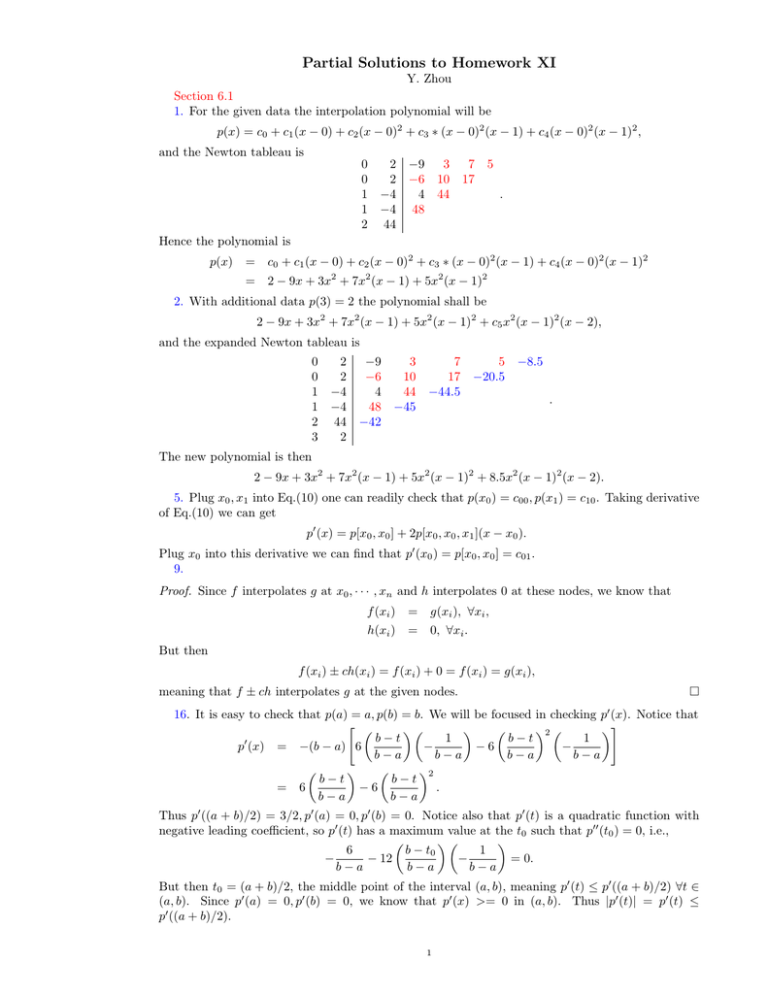
Partial Solutions to Homework XI
Y. Zhou
Section 6.1
1. For the given data the interpolation polynomial will be
p(x) = c0 + c1 (x − 0) + c2 (x − 0)2 + c3 ∗ (x − 0)2 (x − 1) + c4 (x − 0)2 (x − 1)2 ,
and the Newton tableau is
0
2 −9
0
2 −6
1 −4
4
1 −4 48
2 44
3
10
44
7
17
5
.
Hence the polynomial is
p(x)
= c0 + c1 (x − 0) + c2 (x − 0)2 + c3 ∗ (x − 0)2 (x − 1) + c4 (x − 0)2 (x − 1)2
=
2 − 9x + 3x2 + 7x2 (x − 1) + 5x2 (x − 1)2
2. With additional data p(3) = 2 the polynomial shall be
2 − 9x + 3x2 + 7x2 (x − 1) + 5x2 (x − 1)2 + c5 x2 (x − 1)2 (x − 2),
and the expanded Newton tableau is
0
0
1
1
2
3
2 −9
2 −6
−4
4
−4
48
44 −42
2
3
10
44
−45
7
17
−44.5
5
−20.5
−8.5
.
The new polynomial is then
2 − 9x + 3x2 + 7x2 (x − 1) + 5x2 (x − 1)2 + 8.5x2 (x − 1)2 (x − 2).
5. Plug x0 , x1 into Eq.(10) one can readily check that p(x0 ) = c00 , p(x1 ) = c10 . Taking derivative
of Eq.(10) we can get
p0 (x) = p[x0 , x0 ] + 2p[x0 , x0 , x1 ](x − x0 ).
Plug x0 into this derivative we can find that p0 (x0 ) = p[x0 , x0 ] = c01 .
9.
Proof. Since f interpolates g at x0 , · · · , xn and h interpolates 0 at these nodes, we know that
f (xi ) = g(xi ), ∀xi ,
h(xi ) =
0, ∀xi .
But then
f (xi ) ± ch(xi ) = f (xi ) + 0 = f (xi ) = g(xi ),
meaning that f ± ch interpolates g at the given nodes.
16. It is easy to check that p(a) = a, p(b) = b. We will be focused in checking p0 (x). Notice that
" 2 #
b−t
1
b−t
1
0
p (x) = −(b − a) 6
−
−6
−
b−a
b−a
b−a
b−a
2
b−t
b−t
= 6
−6
.
b−a
b−a
Thus p0 ((a + b)/2) = 3/2, p0 (a) = 0, p0 (b) = 0. Notice also that p0 (t) is a quadratic function with
negative leading coefficient, so p0 (t) has a maximum value at the t0 such that p00 (t0 ) = 0, i.e.,
b − t0
1
6
− 12
−
= 0.
−
b−a
b−a
b−a
But then t0 = (a + b)/2, the middle point of the interval (a, b), meaning p0 (t) ≤ p0 ((a + b)/2) ∀t ∈
(a, b). Since p0 (a) = 0, p0 (b) = 0, we know that p0 (x) >= 0 in (a, b). Thus |p0 (t)| = p0 (t) ≤
p0 ((a + b)/2).
1
2
6.4
1,2. Answers were given in class.
5. f (x) is a quadratic spline function because
• f (x) is a polynomial of degree less than or equal to 2 in (−∞, ∞).
• f (x) is continuous in (−∞, ∞). This can be check the value of f (x) at the ends of each
subintervals.
• f 0 (x) is continuous in (−∞, ∞). This can be check the value of 0 f (x) at the ends of each
subintervals.
6. Piecewise polynomial f (x) can be a cubic spline function only if
• f (x) is a polynomial of degree less than or equal to 3 in (−∞, ∞).
• f (x) is continuous in (−∞, ∞). In particular, f (x) must be continuous at the ends of each
subintervals.
• f 0 (x) is continuous in (−∞, ∞). In particular, f 0 (x) must be continuous at the ends of each
subintervals.
• f 00 (x) is continuous in (−∞, ∞). In particular, f 00 (x) must be continuous at the ends of
each subintervals.
By examining these four criterions we get constraints for a, b, c, d, e, i.e.,
a = c = d 6= 0; b 6= 0 or e 6= 0.
Since f (1) = 7, we know c = a = 7. Furthermore, from f (0) = 26 we get b = 2 and from f (4) = 25,
we get e = −3.