Boston University Computer Science Tech. Report No. 2005-017, May, 2005.
To appear in Proc. International Conference on Advanced Video and Signal based Surveillance (AVSS), Sept. 2005.
View Registration Using Interesting Segments of Planar Trajectories
Walter Nunziati1
1
Jonathan Alon2
Stan Sclaroff2
Dipartimento di Sistemi e Informatica
Universitá degli Studi di Firenze
Florence, 50139, Italy.
{nunziati|delbimbo}@dsi.unifi.it
2
Alberto Del Bimbo1
Computer Science Department
Boston University
Boston, MA 02215, U.S.A.
{jalon|sclaroff}@cs.bu.edu
Abstract
We introduce a method for recovering the spatial and temporal alignment between two or more views of objects moving over a ground plane. Existing approaches either assume that the streams are globally synchronized, so that
only solving the spatial alignment is needed, or that the
temporal misalignment is small enough so that exhaustive
search can be performed. In contrast, our approach can recover both the spatial and temporal alignment, regardless of
their magnitude. We compute for each trajectory a number
of interesting segments, and we use their description to form
putative matches between trajectories. Each pair of corresponding interesting segments induces a temporal alignment, and defines an interval of common support across two
views of an object that is used to recover the spatial alignment. Interesting segments and their descriptors are defined using algebraic projective invariants measured along
the trajectories. Similarity between interesting segments is
computed taking into account the statistics of such invariants. Candidate alignment parameters are verified checking
the consistency, in terms of the symmetric transfer error, of
all the putative pairs of corresponding interesting segments.
Experiments are conducted with two different sets of data,
one with two views of an outdoor scene featuring moving
people and cars, and one with four views of a laboratory
sequence featuring moving radio–controlled cars.
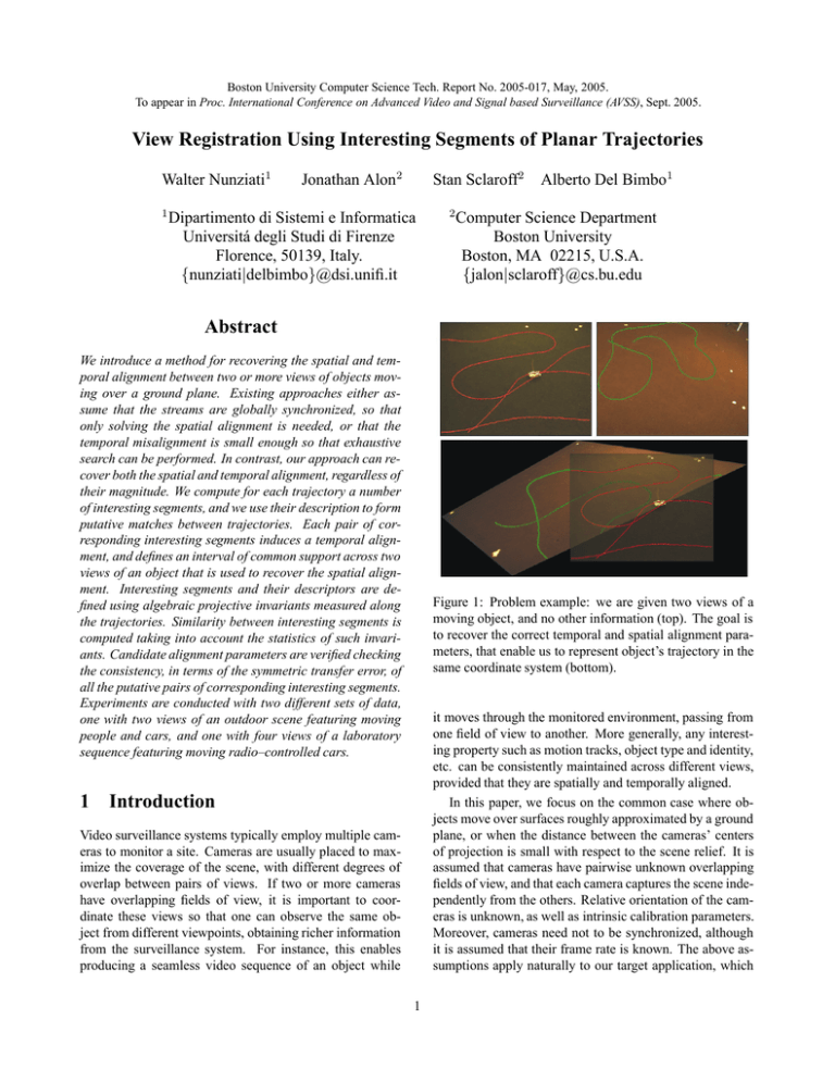
Figure 1: Problem example: we are given two views of a
moving object, and no other information (top). The goal is
to recover the correct temporal and spatial alignment parameters, that enable us to represent object’s trajectory in the
same coordinate system (bottom).
it moves through the monitored environment, passing from
one field of view to another. More generally, any interesting property such as motion tracks, object type and identity,
etc. can be consistently maintained across different views,
provided that they are spatially and temporally aligned.
In this paper, we focus on the common case where objects move over surfaces roughly approximated by a ground
plane, or when the distance between the cameras’ centers
of projection is small with respect to the scene relief. It is
assumed that cameras have pairwise unknown overlapping
fields of view, and that each camera captures the scene independently from the others. Relative orientation of the cameras is unknown, as well as intrinsic calibration parameters.
Moreover, cameras need not to be synchronized, although
it is assumed that their frame rate is known. The above assumptions apply naturally to our target application, which
1 Introduction
Video surveillance systems typically employ multiple cameras to monitor a site. Cameras are usually placed to maximize the coverage of the scene, with different degrees of
overlap between pairs of views. If two or more cameras
have overlapping fields of view, it is important to coordinate these views so that one can observe the same object from different viewpoints, obtaining richer information
from the surveillance system. For instance, this enables
producing a seamless video sequence of an object while
1
is a distributed video surveillance system realized with independent cameras, that requires minimal user effort in the
setup phase.
For the above mentioned case, the geometry of the problem is well known, and consists of estimating the 2D homographies between pairs of overlapping views [15]. The
homography model holds for all the points that are images
of points on the (world) ground plane, either static features,
or points measured along trajectories. For the latter case,
however it must be ensured that correspondences are established on simultaneous points, hence trajectories must be
globally time–aligned across views.
Our method takes as input trajectories in the form of sequences of space–time points (x i (t), y i (t), ti ) for the ith
view, and produces the following output:
ing the search over all the possible time-shifts in order to
recover the correct alignment between two trajectories.
The method has been tested on two datasets acquired in
completely different situations. The first one has been acquired in our laboratory, and consists of radio–controlled
cars moving over a planar scene. The second one is a dataset
made available for the VS–PETS 2001 workshop, consisting of two views of an outdoor scene featuring moving people and cars. In both cases, the computed homographies
produce errors comparable to the tracking errors, and the
recovered time shifts are always within a range of a few
frames with respect to the true ones.
2 Related work
• A set of homographies H ij that spatially maps trajectories in the view i with trajectories in the view j.
The view matching problem described in the previous section has been widely studied. Traditional approaches, well
suited for the case of static scenes, rely on matching a
number N ≥ 4 of static feature points between pairs of
views [2, 5], or determining the correct registration by directly solving a least-squares estimation problem in the unknown structure and motion parameters [3]. These approaches produce accurate results. However, for typical
video-surveillance scenes such methods are not always suitable for several reasons. First, finding a high number of correspondences between widely separated views taken with
different cameras is a difficult problem, since brightness or
proximity constraints do not hold. Moreover, the scene itself may not have enough texture in the region where the
objects move. Finally, one has to be sure that features are
obtained from the ground plane, and not from moving objects and/or other parts of the scene.
Trajectory data on the other hand forms a powerful cue
to obtain correspondences, provided that the trajectories are
time–aligned across views. The basic reasoning is that a
pair of single corresponding trajectories induces multiple
point correspondences. In particular, all the points that belong to the interval of common temporal support of the same
object seen in two views can be used to compute the homography. Usually, a pair of corresponding non–parallel
(in the world) trajectories are sufficient to estimate the correct homography, provided that they span sufficiently well
the region of overlap between the FoVs.
A caveat is that tracking data are usually less accurate
than static scene points obtained with a feature detection algorithm. However, it must be pointed out that the role of
a registration algorithm in the context of a video surveillance system is not that of providing a visually pleasant site
model, but to allow the detection of interesting objects’ correspondences across views. Hence, small registration error
can be easily tolerated. These considerations have been exploited in several works.
• A set of time-shifts ∆ij that temporally align trajectories in the view i with trajectories in the view j.
The set {Hij , ∆ij } for each pair ij, can in turn be used
to express every trajectory point with respect to a common
spatial and temporal coordinate system.
For a pair of views, the method can be outlined as follows: first, trajectories from both views are transformed into
projective invariant sequences of cross ratios; for each point
along a sequence, the statistical properties of the cross ratio
are used to define a measure of saliency of a local trajectory segment centered on the point itself; points that appear to be more interesting according to this measure are
selected together with their support interval, and a table of
putative correspondences between pairs of interesting intervals across the two views is computed based on the invariant
sequence. Each pair of putative correspondences induces a
temporal alignment between two views, and defines an interval of common support that is used to recover the spatial alignment; pairs of putative matches are added to the
homography estimation algorithm, until either there are no
more left, or the estimate does not change significantly; the
latter procedure is repeated for different initial pairs of correspondences, and the resulting homographies are ranked
using the symmetric transfer error; finally, the highest ranking homography is selected.
The major contribution of this work is a method that recovers spatial–temporal alignment between two views of
the same scene regardless of the actual amount of misalignment, both in space and time. This is achieved by introducing the concept of salient segments of a trajectory. Being
based on the cross-ratio of five coplanar points, the measure
is invariant with respect to changes in viewpoint. Salient
trajectory points provide a sparse representation of the trajectories that is used to initialize the correspondence, avoid2
p represent the spatial coordinates of the point in the two
views in homogeneous coordinates.
The first attempt to estimate the homography and the
time–shift using tracking data was been presented in [11].
Motion data were treated as unordered sets of points, and
not as trajectories. In [7], a method was presented for estimating both planar and non–planar correspondence models,
and to take advantage of the tracking sequences rather than
just co–occurring object detections. This resulted in a more
reliable estimation. However, temporal alignment was recovered by exhaustive search over a small, fixed temporal
interval, which is not a suitable approach when sequences
are widely separated in time.
In [4], cameras were assumed to be calibrated, and temporal alignment was recovered by exhaustive search, using
a least median of square scores of the results. Khan et al.
[9] automatically estimated the line where the feet of pedestrians should appear in a secondary camera when they exit
the reference camera. This assumes that objects exit the
scene at a linear occlusion boundary, and information is collected only when objects actually cross the fields of view
lines. Color information acquired from moving objects was
used in [10], to detect objects’ correspondences between
views taken with pan–tilt–zoom synchronized cameras, a
setup which is fundamentally different from ours. In [13]
synchronized cameras was used to recover the correspondence model both for the cases of overlapping and non–
overlapping views.
Our approach builds on the work of [7] for the case of
planar scenes, and improves on the existing work in two
directions: tentative corresponding pairs of trajectories are
initialized using a local measure of saliency, allowing the
system to deal with the case of partial overlapping view; furthermore, time–shift between trajectories can be arbitrary,
and the amount of the time shift does not affect the complexity of the algorithm. We exploit intrinsic properties of
the trajectories, defining a representation which is invariant
to changes in view–point. This idea is inspired by works on
model–based object recognition using algebraic and semi–
differential projective invariants [14, 12, 6], adapted for the
particular case of representing trajectories. In particular, our
representation can deal with configurations of three or more
collinear points, a common situation that occurs along a trajectory of a pedestrian or a car.
3.1 Invariant trajectory representation
We begin by transforming each trajectory in the two views
to a representation which is invariant to changes in view
point. Output of an object tracker is assumed. The points
are first locally smoothed using a cubic spline fitted via least
squares. The method is sketched in Fig.2, and is based on
the cross ratio of five coplanar points:
τ=
|m125 ||m134 |
,
|m124 ||m135 |
where mijk = (pi , pj , pk ) with pi = (x(t), y(t), 1)t and
|m| is the determinant of m. The point p 1 is the reference
point. For each point p(t) along the curve, four other points
p(t − 2k), p(t − k), p(t + k), p(t + 2k) are used to compute a cross ratio. The parameter k is a time interval that
controls the scale at which the representation is computed.
The greater is k, the less local the representation. With respect to Fig. 2, points p(t−2k), p(t−k), p(t+k), p(t+2k)
are used to compute the point q, and then the intersection between the lines defined by segments p(t), q and
p(t − 2k), p(t + 2k) is chosen to be the reference point
r(t) for the cross ratio. If four collinear points are detected,
the representation is obtained using the cross ratio of these
points. The sequence of image coordinates (x(t), y(t)) is
then transformed into a (view–invariant) sequence of cross
ratios s(t) of the form:
s(t) = τ5 (r(t), p(t − k), p(t), p(t + k), p(t + 2k)),
where the function τ 5 (p1 , p2 , p3 , p4 , p5 ) is the five point
cross ratio. If collinearity has been detected, we set:
s(t) = τ4 (p(t − k), p(t), p(t + k), p(t + 2k)),
where τ4 (p1 , p2 , p3 , p4 ) is the cross ratio of four collinear
points. The described transformation is projective invariant,
since it is based on collinearity and intersection between
points.
3 Approach
3.2 Detecting salient trajectory points
From now on we focus on the case of recovering the temporal and spatial registration parameters for a pair of partially
overlapping views a and b. This is the fundamental instance
of our problem (Fig.1). Under the planar trajectory assumption, and if video streams are not temporally aligned, the
space–time relation between a point visible in both cameras
is expressed by an unknown 3 × 3 homography H and an
unknown time–shift ∆t: Hp(t) = p (t + ∆t), where p and
Being based on the cross ratio, the representation described
above has some significant statistical properties. In particular, it can be shown [1] that under general conditions
the cross ratio has a nonuniform probability density function p(x), shown in Fig. 3. We use this fact to compute a
saliency measure for each sample of the invariant trajectory
representation. This measure is defined in terms of the entropy of the invariant sequence for an interval centered on a
3
p(ti+k)
p(ti+k)
p(ti)
p(ti+2k)
l1
p(ti-k)
l2
p(ti)
p(ti-k)
q
l3
each pair of views a, b, where n a and nb are the numbers
of interesting salient points detected in the two views. Let
Pia , Pjb , tai , tbj , i = [1 . . . na ], j = [1 . . . nb ] represent interesting points and their time indices in the two views. Each
entry of the table contains the similarity measure for a pair
of intervals:
p(ti+2k)
l4
r(ti)
r(ti)
p(ti-2k)
p(ti-2k)
b
ta
i +l,tj +l
ab
Sij
p(s(j)) log2 (
j=t−l
d(sa (ja ), sb (jb )),
where sa , sb are two invariant representation of trajectories, and d(sa (ja ), sb (jb )) is the distance between two cross
ratios with respect to the cumulative distribution function
F (x) shown in Fig. 3. If x 1 and x2 are two cross ratios,
their distance is defined as follows:
point s(t):
j=t+l
=
ja =ta
−l,jb =tbj −l
i
Figure 2: Left) The construction used in our method to compute cross ratios along the trajectory. Right) The five points
cross ratio that constitutes the invariant representation of a
point p(tk ) in the general case.
e(t) =
=
dist(Pia , Pjb )
d(x1 , x2 ) = min(|F (x1 ) − F (x2 )|, 1 − |F (x1 ) − F (x2 )|)
1
),
p(s(j))
This measure has the property of stretching differences
of cross ratios of big values, which are known to be less
stable. Moreover, it takes into account the symmetric properties of cross ratios, in particular the fact that there are two
ways to go from one cross ratio to another: one passing
through the real line, and the other through the point at infinity [8]. We have verified experimentally that the invariant feature described above obeys the distribution of Fig. 3,
although input points are not exactly independent. An example of the matching process is given in Fig. 4.
where l is half the width of the interval. This measure represents in a compact, view–invariant way the local properties
of the trajectory, in terms of curvature, speed, and overall
shape. It is natural to assume that peaks in the sequence
e(t) correspond to the “most informative” points of the trajectory p(t) = (x(t), y(t)). Peaks are found by direct comparison of a value e(t) with its neighbors. Every point of
the trajectory corresponding to a peak, and its surrounding
interval of length 2l, are defined to be an interesting point
and an interesting segment of the sequence, respectively.
180
150
160
140
100
1
0.9
y (pixel)
y (pixel)
120
100
80
p(x)
50
0.8
60
t’=167
F(x)
40
0.7
t=145
(a)
0.6
0.5
0
50
100
150
200
x (pixel)
250
300
350
(b)
0
0
50
100
150
200
250
300
350
x (pixel)
Figure 4: a) First partial view of a trajectory - b) Second
partial view of a trajectory. Boxes indicate detected salient
points. The two filled boxes are found similar, and this correspondence induces an alignment between frame 145 in the
first view with frame 167 in the second view.
0.4
0.3
0.2
0.1
0
−5
20
−4
−3
−2
−1
0
1
2
3
4
5
x (cross ratio)
Figure 3: The probability density function p, and the cumulative density function F of the cross ratio.
3.4 Homography estimation
Each pair of interest points P ia , Pjb induces a temporal
alignment between the trajectories they belong to (Fig. 4).
The alignment is defined by the time–shift obtained by
the difference of the time indices of the interesting points:
∆ti,j = tai − tbj . This in turn defines a temporal interval
of mutual support, i.e., the temporal interval in which the
two trajectories appears in the region of overlap if the time
correspondence is valid. This interval is computed as follows. Let T1 ∈ a, T2 ∈ b, be the two trajectories which are
3.3 Forming putative correspondences
Interesting points from the two views, and their relative support intervals are used to establish space-time pairwise correspondences between trajectories. The method follows the
line of the automatic homography estimation algorithm of
[15]. In particular, a table S ab of size na × nb is formed for
4
hypothesized to correspond. Their spatial–temporal relation can now be expressed as: T 1 (x(t), y(t)) = T2 (x(t +
∆ti,j , y(t + ∆ti,j ), where t is now a common time index.
Now if [t1s , t1f ] and [t2s , t2f ] are the first and the last time indices of the two trajectories on this common time line, the
interval of common support between T 1 and T2 is simply
defined by U = [t 1s , t1f ] ∩ [t2s , t2f ].
All the points of T1 and T2 that fall into the interval
U are fed into the DLT algorithm [15] for estimating the
homography. The process of selecting putative pairs of trajectories, and finding their interval of common support is
iterated until either there are no more putative pairs left, or
the estimated homography does not change. At this point,
the symmetric transfer error is evaluated to verify the result
of the registration:
d(pi , H −1 (pi + ∆t))2 + (Hpi , pi + ∆t)2 .
err =
global view. In any case, the objective is to set the amount
of smoothing such that the obtained table of putative correspondences is as stable as possible. Good results were
achieved smoothing trajectories of cars and pedestrian with
cubic splines with two control points every 30 observations.
4 Results
The proposed method was tested on two datasets. The first
type of data was obtained in our laboratory, using three uncalibrated cameras with partial overlap between the fields
of view. The moving objects consisted of three radio controlled toy cars, and the scene was globally planar. The
camera lenses were selected to reduce the effect of nonlinear distortions. To verify the robustness of the method
to scale changes, different zoom factors were adopted for
each camera. Six trials were conducted with different setups, in terms of FoVs overlap, camera placement/zoom,
and objects’ motion. For each trial, one minute of video at
30 frames per second was acquired for each camera, allowing the cars to move through the overlapping zone several
times. k = l = 15 in this and the next experiment.
The results are well represented by the example shown
in Fig. 5. On average, about 5–10 interesting points were
detected on each trajectory. With respect to the ground
truth, minimum, maximum and average error of the recovered time shift were respectively 7, 16 and 10.2 frames. A
refinement procedure was run over a small interval of 50
frames centered on the recovered solution, checking all the
possible alignments. Typically, a slightly better alignment
was found, and the average error was reduced to 4 frames.
The spatial alignment was always effectively unchanged.
In all the experiments the space–time alignment obtained
with the presented method was sufficient to determine objects’ correspondences across views, which is the goal of
this work. If more accurate registration is needed, for example to build a visually pleasant site model, a refinement
procedure can be carried out, starting from the approximate
solution obtained from correspondences of static scene features. In fact, it was observed that, below a certain limit, the
tracking error becomes the limiting factor of an approach
based on trajectory data. A global re–estimation of the common coordinate system would as well improve on the initial
solution [5].
In the second experiment, a dataset of two views of a typical outdoor surveillance scene, provided for the VS–PETS
2001 workshop was used 1 . This was a more challenging
task, because trajectories were less complicated than those
of the first experiments, and because of the wide variation in
viewpoint and scale. A subset of three trajectories per view
i
The above procedure is repeated for various initial putative
pairs, and the homography that produces the smallest error
is selected.
3.5 Parameter setting
The method described above has a few data–dependent parameters whose choice has been determined experimentally.
Some intuition behind these choices is provided here. In
particular, the two parameters k and l of Sect. 3.1 and 3.2,
and the amount of smoothing that is applied to the data have
impact on the invariant representation, which in turn affects
the location and description of the salient points.
The parameter k controls the locality of the representation. In principle, a small k is desirable, since it would give
a more local representation for matching partial trajectory
segments. However, this must be traded–off with the informative content of the resulting transformed sequence, since
on smaller scale the cross ratios tend to assume very similar
values. In our experiment, we verified that for objects like
people and cars, a good choice is to select k approximately
equal to half the frame rate. For instance, if frame rate is
30 fps, we set k = 15. The algorithm is quite insensitive
to the choice of the parameter l. In fact, we have verified
that small variations of this parameter do not produce big
changes in the location and values of the peak of the entropy
sequence. Furthermore, even if such changes are observed,
they are consistent across views, so corresponding interest
points can still be found. In our experiment, we set l = k.
The amount of smoothing applied prior to the computation of the invariant representation appears to be more
critical. In general, this is mainly due to the well–known
instability of the cross ratio. In particular, problems happen when there are substantial differences in scale between
two views, e.g. a close–up of a part of the scene and a
1 The
sequence and the tracking data are available
http://peipa.essex.ac.uk/ipa/pix/pets/PETS2001/DATASET1/
5
at
Figure 6: Registration results for the two views PETS sequence.
was provided to the algorithm. Fig. 6 shows the obtained
results. With respect to a ground–truth alignment manually obtained carefully selecting corresponding pairs of static feature points, the overall spatial error was 3.4 pixels,
with a variance of 7.9 pixels. The time shift was recovered
with an error of 9 frames. Further refinement using trajectory data does not improved significantly on this first solution. Although mis–registration errors are clearly visible
in Fig. 6, the solution was definitely sufficient to compare
trajectories of objects in the recovered common coordinate
frame, to understand if two trajectories in different views
correspond to the same 3D object.
poral misalignment is known or small enough so that exhaustive search can performed. In contrast, the proposed
approach is based on the concept of interesting trajectory
points/segments, that allow to recover both spatial and temporal alignment, independently on the magnitude of both.
The method enable to solve the problem of understanding correspondences between moving objects across views.
Furthermore, the method can also be used in tasks where
sub–pixel and sub–frame registration is needed, to efficiently found a solution that can be used to initialize a refinement registration technique, such as [5]. In fact, although the recovered solution is generally an approximation of the ideal alignment, it must be pointed out that very
simple assumptions are needed, namely knowing the relative frame rate, and observing a limited number of trajectories simultaneously. Since it has been observed that the
precision of the method is ultimately limited by the performance of the tracker, we argue that the refinement procedure should be based on the analysis of static scene features, and should be followed by a global re–estimation of
the spatial parameters for the case of more than two views.
References
Figure 5: One example of the registration results for a three
views car sequence. The reference view correspond with the
one in the center of the figure. Big registration errors are due
to either tracking errors in one view, or to error propagation
between homographies. For instance, in the zone outlined
with the yellow circle, in one view the tracker was fooled
by the shadow of the object.
[1] K. Åstrom and L. Morin. “Random Cross Ratios”. Report RT
88 IMAG–LIFIA, 1992.
[2] A. Baumberg. “Reliable feature matching across widely separated views”. In Proc. of CVPR, 2000.
[3] J. Bergen, P. Anandan, and M. Irani. “Efficient Representation
of Video Sequences and Their Applications”. Signal Processing: Image Communication, 1999.
[4] J. Black, T. Ellis, P. Rosin. “Multi View Image Surveillance
and Tracking”. In Proc. of MOTION Workshop, 2002.
5. Conclusions
[5] M. Brown and D. G. Lowe. “Recognising Panoramas”. In
Proc. of ICCV, 2003.
A method for recovering the time–alignment and the spatial registration between different views of planar trajectory data has been presented. We overcome the limitations of existing methods, which typically assume that tem-
[6] S. Carlsson, R. Mohr, T. Moons, L. Morin, et.al. “Semi-Local
Projective Invariants for the Recognition of Smooth Plane
Curves”. International Journal of Computer Vision, 1996.
6
[7] Y. Caspi, D. Simakov, and M. Irani. “Feature-Based
Sequence-to-Sequence Matching”. Proc. of VMODS Workshop, 2002.
[8] P. Gros. “How to Use the Cross Ratio to Compute Projective
Invariants from Two Images”. Proc. of Application of Invariance in Computer Vision, 1993.
[9] S. Khan and M. Shah. “Consistent Labeling of Tracked Objects in Multiple Cameras with Overlapping Fields of View”.
IEEE TPAMI, 2003.
[10] J. Kang, I. Cohen, and G. Medioni. “Multi-Views Tracking
Within and Across Uncalibrated Camera Streams”. In Proc. of
ACM SIGMM 2003 Workshop on Video Surveillance, 2003.
[11] L. Lee, R. Romano, and G. Stein. “Monitoring Activities
from Multiple Video Streams: Establishing a Common Coordinate Frame”. IEEE TPAMI, 2000.
[12] J. Mundy and A. Zisserman, editors. “Geometric Invariance
in Computer Vision”. MIT Press, Cambridge, MA, 1992.
[13] C. Stauffer and K. Tieu. “Automated multi-camera planar
tracking correspondence modeling”. Proc. of CVPR, 2003.
[14] L. Van Gool, P. Kempenaers, and A. Oosterlinck. “Recognition and semi-differential invariants”. Proc. of CVPR, 1991.
[15] R. Hartley and A. Zisserman. “Multiple View Geometry in
Computer Vision”, Cambridge University Press, 2004.
7