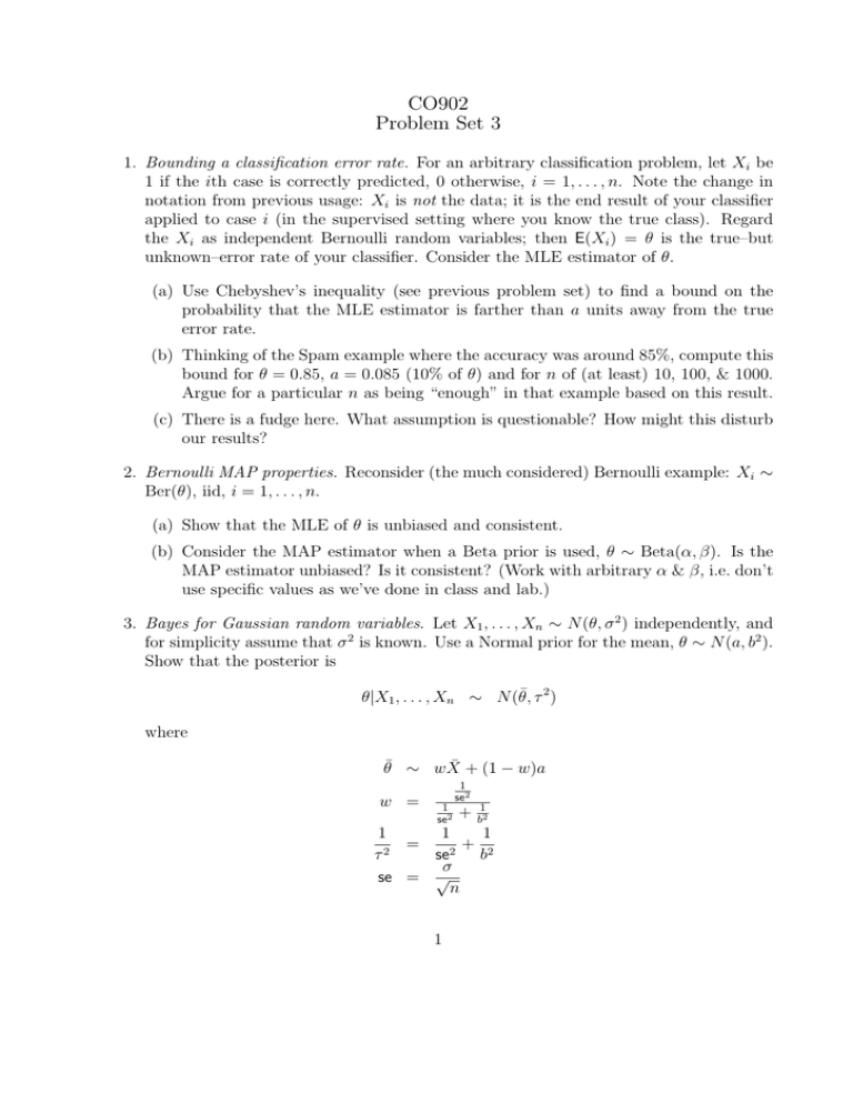
CO902
Problem Set 3
1. Bounding a classification error rate. For an arbitrary classification problem, let Xi be
1 if the ith case is correctly predicted, 0 otherwise, i = 1, . . . , n. Note the change in
notation from previous usage: Xi is not the data; it is the end result of your classifier
applied to case i (in the supervised setting where you know the true class). Regard
the Xi as independent Bernoulli random variables; then E(Xi ) = θ is the true–but
unknown–error rate of your classifier. Consider the MLE estimator of θ.
(a) Use Chebyshev’s inequality (see previous problem set) to find a bound on the
probability that the MLE estimator is farther than a units away from the true
error rate.
(b) Thinking of the Spam example where the accuracy was around 85%, compute this
bound for θ = 0.85, a = 0.085 (10% of θ) and for n of (at least) 10, 100, & 1000.
Argue for a particular n as being “enough” in that example based on this result.
(c) There is a fudge here. What assumption is questionable? How might this disturb
our results?
2. Bernoulli MAP properties. Reconsider (the much considered) Bernoulli example: Xi ∼
Ber(θ), iid, i = 1, . . . , n.
(a) Show that the MLE of θ is unbiased and consistent.
(b) Consider the MAP estimator when a Beta prior is used, θ ∼ Beta(α, β). Is the
MAP estimator unbiased? Is it consistent? (Work with arbitrary α & β, i.e. don’t
use specific values as we’ve done in class and lab.)
3. Bayes for Gaussian random variables. Let X1 , . . . , Xn ∼ N (θ, σ 2 ) independently, and
for simplicity assume that σ 2 is known. Use a Normal prior for the mean, θ ∼ N (a, b2 ).
Show that the posterior is
θ|X1 , . . . , Xn ∼ N (θ̄, τ 2 )
where
θ̄ ∼ wX̄ + (1 − w)a
w =
1
se2
1
se2
+
1
b2
1
1
1
=
+
τ2
se2 b2
σ
se = √
n
1
Inverse variance is also known as precision; what role does the prior precision and data
precision play in w? What role doe they play in the posterior precision? What happens
as n grows?
4. Iterated Expectation & Variance. Prove these two fundamental and incredibly useful
identities. For continuous random variables X and Y with joint distribution p(x, y)
and marginal distributions p(x) and p(y),
E(X) = EY (EX (X|Y ))
Var(X) = EY (VarX (X|Y )) + VarY (EX (X|Y ))
The subscripts remind you how to compute each expectation or variance. In the
expression X|Y , the random variable Y is “conditioned upon” and thus there is no
randomness in Y , and thus any expectation must be w.r.t. X alone (EX ). For EX (X|Y ),
note that anR expectation with respect to X integrates out all dependence on X (i.e.
the integral · p(x)dx cannot depend on x), and so EX (X|Y ) can only depend on Y
(and thus EY ). The same goes with the second expression with the variances.
Note that these expressions are actually unambiguous with out the subscripts—there
is only one way you can evaluate them—but the subscripts help ‘lead the way’.
TEN / January 28, 2013
2