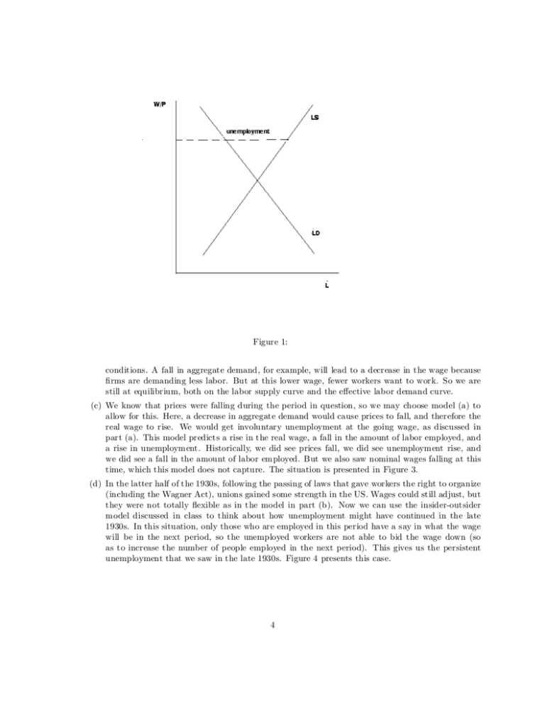
Figure 1:
conditions. A fall in aggregate demand, for example, will lead to a decrease in the wage because
¯rms are demanding less labor. But at this lower wage, fewer workers want to work. So we are
still at equilibrium, both on the labor supply curve and the e®ective labor demand curve.
(c) We know that prices were falling during the period in question, so we may choose model (a) to
allow for this. Here, a decrease in aggregate demand would cause prices to fall, and therefore the
real wage to rise. We would get involuntary unemployment at the going wage, as discussed in
part (a). This model predicts a rise in the real wage, a fall in the amount of labor employed, and
a rise in unemployment. Historically, we did see prices fall, we did see unemployment rise, and
we did see a fall in the amount of labor employed. But we also saw nominal wages falling at this
time, which this model does not capture. The situation is presented in Figure 3.
(d) In the latter half of the 1930s, following the passing of laws that gave workers the right to organize
(including the Wagner Act), unions gained some strength in the US. Wages could still adjust, but
they were not totally °exible as in the model in part (b). Now we can use the insider-outsider
model discussed in class to think about how unemployment might have continued in the late
1930s. In this situation, only those who are employed in this period have a say in what the wage
will be in the next period, so the unemployed workers are not able to bid the wage down (so
as to increase the number of people employed in the next period). This gives us the persistent
unemployment that we saw in the late 1930s. Figure 4 presents this case.
4
Figure 2:
5
Figure 3:
6
Figure 4:
7