A note on the random greedy triangle-packing algorithm
Tom Bohman, Alan Frieze and Eyal Lubetzky
(These notes were prepared by Lutz Warnke, warnke@maths.ox.ac.uk)
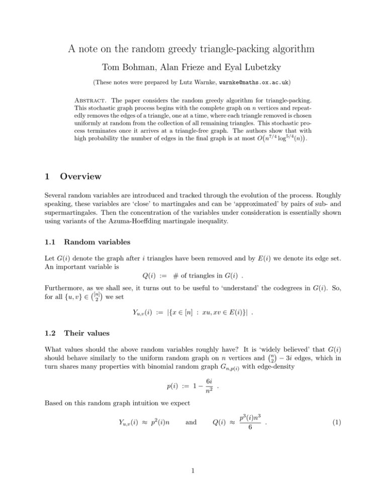
Abstract. The paper considers the random greedy algorithm for triangle-packing.
This stochastic graph process begins with the complete graph on n vertices and repeatedly removes the edges of a triangle, one at a time, where each triangle removed is chosen
uniformly at random from the collection of all remaining triangles. This stochastic process terminates once it arrives at a triangle-free graph. The authors show that with
high probability the number of edges in the final graph is at most O n7/4 log5/4 (n) .
1
Overview
Several random variables are introduced and tracked through the evolution of the process. Roughly
speaking, these variables are ‘close’ to martingales and can be ‘approximated’ by pairs of sub- and
supermartingales. Then the concentration of the variables under consideration is essentially shown
using variants of the Azuma-Hoeffding martingale inequality.
1.1
Random variables
Let G(i) denote the graph after i triangles have been removed and by E(i) we denote its edge set.
An important variable is
Q(i) := # of triangles in G(i) .
Furthermore, as we
shall see, it turns out to be useful to ‘understand’ the codegrees in G(i). So,
for all {u, v} ∈ [n]
2 we set
Yu,v (i) := |{x ∈ [n] : xu, xv ∈ E(i)}| .
1.2
Their values
What values should the above random variables roughly have? It is ‘widely
believed’ that G(i)
should behave similarly to the uniform random graph on n vertices and n2 − 3i edges, which in
turn shares many properties with binomial random graph Gn,p(i) with edge-density
p(i) := 1 −
6i
.
n2
Based on this random graph intuition we expect
Yu,v (i) ≈ p2 (i)n
and
1
Q(i) ≈
p3 (i)n3
.
6
(1)
1.3
Expected one-step changes
Observe that with Yu,v (i) we can express the one-step change of Q(i) as follows: if the (i + 1)-th
triangle taken is abc then
Q(i) − Q(i + 1) = Ya,b (i) + Yb,c (i) + Ya,c (i) − 2 .
With this in mind, after conditioning on the first i steps, the expected one-step change of Q(i) is
given by
E[Q(i + 1) − Q(i) | G(i)] = −
X
xyz∈Q(i)
Yxy (i) + Yxz (i) + Yyz (i) − 2
Q(i)
X
1
= 2−
Q(i)
(2)
2
Yxy (i) ,
xy∈E(i)
P
where we also have 3Q(i) = xy∈E(i) Yxy (i). But why is this useful? Well, Q(i) can essentially be
‘transformed’ to sub- and supermartingales by adding or subtracting appropriate functions. Then
(modulo some technical details) the concentration follows from Azuma-Hoeffding type martingale
inequalities.
We remark that the same strategy also applies to Yu,v (i); but here the details are more involved.
1.4
Main Result
Loosely speaking, the main technical result states that during the first
5
1
i∗ := n2 − n7/4 log5/4 (n)
6
3
(3)
steps the approximations given by (1) hold whp. Note that Q(i∗ ) = ω(1), and thus the process has
not terminated yet; so whp the final graph of the random process has
n
− 3i∗ = O(n7/4 log5/4 (n))
2
edges, which implies their main result.
1.5
Remark
In the current proof the bound (3) is ‘limited’ by the way in which the concentration of Yu,v (i) is
shown. In fact, the authors claim that with a more sophisticated analysis (and introducing more
random variables) they are able to reduce the final number of edges to roughly O(n1.65+o(1) ). Finally,
it is widely believed that whp the final graph has n3/2+o(1) edges (Joel Spencer has offered $200 for
a resolution of this question).
2