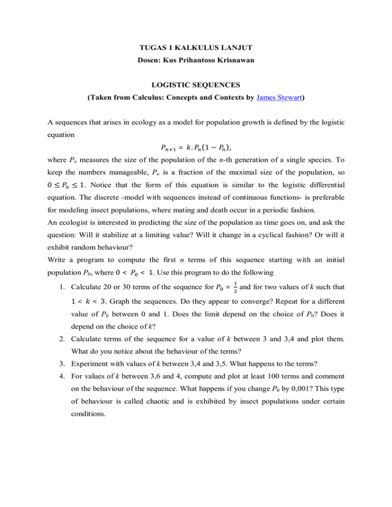
TUGAS 1 KALKULUS LANJUT
Dosen: Kus Prihantoso Krisnawan
LOGISTIC SEQUENCES
(Taken from Calculus: Concepts and Contexts by James Stewart)
A sequences that arises in ecology as a model for population growth is defined by the logistic
equation
= .
(1 −
),
where Pn measures the size of the population of the n-th generation of a single species. To
keep the numbers manageable, Pn is a fraction of the maximal size of the population, so
0≤
≤ 1. Notice that the form of this equation is similar to the logistic differential
equation. The discrete -model with sequences instead of continuous functions- is preferable
for modeling insect populations, where mating and death occur in a periodic fashion.
An ecologist is interested in predicting the size of the population as time goes on, and ask the
question: Will it stabilize at a limiting value? Will it change in a cyclical fashion? Or will it
exhibit random behaviour?
Write a program to compute the first n terms of this sequence starting with an initial
population P0, where 0 <
< 1. Use this program to do the following
1. Calculate 20 or 30 terms of the sequence for
1<
= and for two values of k such that
< 3. Graph the sequences. Do they appear to converge? Repeat for a different
value of P0 between 0 and 1. Does the limit depend on the choice of P0 ? Does it
depend on the choice of k?
2. Calculate terms of the sequence for a value of k between 3 and 3,4 and plot them.
What do you notice about the behaviour of the terms?
3. Experiment with values of k between 3,4 and 3,5. What happens to the terms?
4. For values of k between 3,6 and 4, compute and plot at least 100 terms and comment
on the behaviour of the sequence. What happens if you change P0 by 0,001? This type
of behaviour is called chaotic and is exhibited by insect populations under certain
conditions.