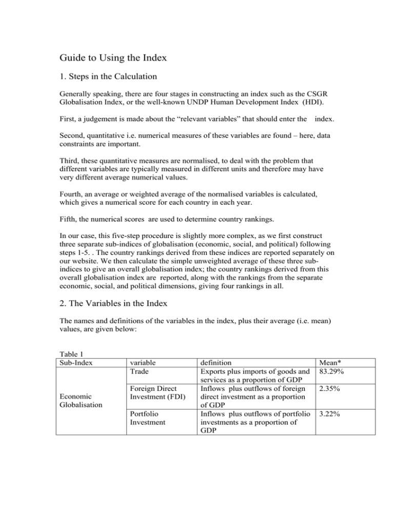
Guide to Using the Index
1. Steps in the Calculation
Generally speaking, there are four stages in constructing an index such as the CSGR
Globalisation Index, or the well-known UNDP Human Development Index (HDI).
First, a judgement is made about the “relevant variables” that should enter the index.
Second, quantitative i.e. numerical measures of these variables are found – here, data
constraints are important.
Third, these quantitative measures are normalised, to deal with the problem that
different variables are typically measured in different units and therefore may have
very different average numerical values.
Fourth, an average or weighted average of the normalised variables is calculated,
which gives a numerical score for each country in each year.
Fifth, the numerical scores are used to determine country rankings.
In our case, this five-step procedure is slightly more complex, as we first construct
three separate sub-indices of globalisation (economic, social, and political) following
steps 1-5. . The country rankings derived from these indices are reported separately on
our website. We then calculate the simple unweighted average of these three subindices to give an overall globalisation index; the country rankings derived from this
overall globalisation index are reported, along with the rankings from the separate
economic, social, and political dimensions, giving four rankings in all.
2. The Variables in the Index
The names and definitions of the variables in the index, plus their average (i.e. mean)
values, are given below:
Table 1
Sub-Index
Economic
Globalisation
variable
Trade
Foreign Direct
Investment (FDI)
Portfolio
Investment
definition
Exports plus imports of goods and
services as a proportion of GDP
Inflows plus outflows of foreign
direct investment as a proportion
of GDP
Inflows plus outflows of portfolio
investments as a proportion of
GDP
Mean*
83.29%
2.35%
3.22%
Income
People
Foreign Stock
Foreign Flow
Social
Globalisation
Worker
Remittances
Tourists
Ideas
Phone calls
Internet users
Films
Books and
newspapers
Mail
Embassies
Political
Globalisation
UN Missions
Organisations
Employee compensation paid to
non-resident workers and
investment income from foreign
9.12%
assets owned by domestic
residents plus employee
compensation paid to resident
workers working abroad and
investment income from domestic
assets owned by foreign residents,
as a proportion of GDP.
Stock of foreign population as
proportion of total population.
Inflows of foreign population as
proportion of total population.
Worker remittances (receipts) as a
proportion of GDP.
Number of tourists (arrivals plus
departures) as proportion of total
population.
6.65%
International outgoing telephone
traffic (minutes) per capita
Internet users as a percentage of
population
Number of films imported and
exported.
Sum of value of books and
newspapers imported and exported
per capita (US dollars)
Number of international letters
delivered and sent per capita
0.059
Number of foreign embassies in
country
Number of UN peacekeeping
operations in which country
participates
Number of memberships of
International organisations
34.16
0.5%
3.11%
57.15%
3.97%
310.92
10.08
15.76
1.16
40.70
* Calculated over all countries/years
So, the economic globalisation index is constructed from four variables, the social
globalisation index is constructed from nine variables (four included in the people
globalisation sub-index, and five in the ideas globalisation sub-index), and the
political globalisation index is constructed from three variables.
It is also clear from Table 1 that the mean or average values of the variables differ
considerably, even across variables that are used to construct a given sub-index. To
deal with this, we normalise the variables.
3. The Sources of Data
The variables in the index are taken from a variety of data sources, as indicated in the
Table below.
Table 2
Sub-Index
Variables
Source
Trade
World Bank- World Development Indicators - Latest
issue
FDI
World Bank- World Development Indicators - Latest
Economic
issue
Globalisation
Portfolio
IMF- International Financial Statistics- Latest issue
Investment
Income
World Bank- World Development Indicators- Latest
issue
People
Foreign Stock
Foreign Flow
Social
Globalisation
Worker
Remittances
Tourists
Ideas
Phone calls
Internet users
Films
Political
Globalisation
World Bank- World Development Indicators- Latest
issue
World Bank- World Development Indicators- Latest
issue, and Mitchell, B. R. 1998. International
Historical Statistics. New York: Stockbridge Press
and London: Macmillan.
World Bank- World Development Indicators- Latest
issue
World Bank- World Development Indicators- Latest
issue
International Telecommunication Union (ITU)
World Telecommunication Indicators Database
(www.itu.int)
International Telecommunication Union (ITU)
World Telecommunication Indicators Database
(www.itu.int)
UNESCO -1999 Statistical Yearbook
(www.unesco.org)
Books and
newspapers
Mail
UNESCO-1999 Statistical Yearbook
(www.unesco.org)
Universal Postal Union (www.upu.int)
Embassies
Europa World Yearbook- various years. (Latest issue
available on line for subscribers at
(http://www.europaworld.com.))
UN Missions
Organisations
CIA- World Factbooks, various years. (Latest issue
available on line at
(http://www.cia.gov/cia/publications/factbook/))
United Nations Website (www.un.org)
CIA- World Factbooks, various years. (Latest issue
available on line at
(http://www.cia.gov/cia/publications/factbook/))
4. Normalisation
The method we use is panel normalisation. To illustrate, suppose the variable is trade.
First, the minimum and maximum values of this variable over the years 1970-2001,
and over all countries, are found. In the case of the trade variable, it turns out that the
maximum is 1448 %, for Netherlands Antilles in 1980, and the minimum is 6%, for
Sudan in 1987. Then, if the trade variable for some country (say the UK) in some year
is x%, then the panel normalised value of x is
y = (x – 6)/(1448-6)
Note that with this normalisation, all values of y lie between zero and one. Note also
that, with this method, the means and the variances of different variables can still be
different to each other, although they will be much closer to each other than before
panel normalisation.
Panel normalisation has both advantages and disadvantages. The advantage is that
with panel-normalised data, we can make meaningful comparisons over time for a
given country or indeed between countries. A disadvantage, discussed in detail in
Lockwood (2004), is that when additional years of data are added to the database, the
maximum or minimum value of a variable may change, and those variables affected
then have to be re-normalised. For example, suppose Sudan’s trade openness variable
rose from 6% to 10% in 1987; from the above formula in Section 2, this would
change the value of trade openness for the UK in (say) 1998. This changes countries’
scores in previous years, and could even change their ranking in the overall
globalization index in previous years.
Nevertheless, a major objective in constructing our index is to make comparisons
between different points in time. So, in spite of the problem just discussed, we use
panel normalisation.
5. Weighting
Once the different variables in the index have been normalised, they have to be
“added together” to generate the index. At this point, there are two alternatives.
First, the index can be constructed by taking a simple average of the variables. This is
straightforward, but of course imposes the assumption that all variables entering the
index are equally important.
Second, the index can be constructed by taking a weighted average of the variables,
where the weights are positive and add up to one. There are then two ways of
assigning the weights.
First, the weights can be subjective, i.e. chosen by the researcher according to his/her
subjective belief about which variables are more important. This is the approach taken
by Foreign Policy and A.T.Kearney in the construction of their Globalisation Index.
In fact, in the latest version of their index, they double-weight FDI flows, as they
believe that this is a particularly important indicator of globalisation.
Second, the weights can be chosen to maximise the informativeness of the index:
statistically optimal weights. We take the second approach, as we feel this avoids any
subjective bias on the part of the researcher as to which weights are important.
Briefly, statistically optimal weighting (or principal component weighting, as it is
more properly known) works as follows (if you want to know more, see the
Appendix!). Take for example, the four variables that make up the economic
globalisation index. In 2000, these were available for 119 countries. Thus, in 2000, we
are using 119x4 pieces of information. When we aggregate these four variables to
make the index, we end up with only one piece of information about each country:
thus we are “throwing away” 119x3 pieces of information. Statistically optimal
weighting ensures that when we do this, we retain as much as possible of the original
information about the countries.
The statistically optimal weights used in the construction of our index are:
Table 3
Sub-Index
Economic
Globalisation
Social
Globalisation
variables
Trade
Fdi
Portfolio
Income
weight
0.418
0.092
0.220
0.270
People
Foreign Stock
Foreign Flow
Worker
Remittances
0.331
0.266
0.629
0.079
0.026
Tourists
Ideas
Phone calls
Internet users
Films
Books and
newspapers
Mail
Political
Globalisation
0.669
0.004
0.303
0.061
0.577
0.054
Embassies
0.378
UN Peace Missions 0.357
International
0.266
Organisations
Note that weights sum to one for each of the sub-indices.
6. Controlling for Fixed Country Characteristics
A final refinement in the construction of our index is the following. Broadly speaking,
the variables used in our index to measure different dimensions of globalisation
measure outcomes, rather than policy. For example, the variable they use to measure
openness to trade is the value of total trade (imports plus exports) as a percentage of
GDP.
A well-known problem with this measure of trade openness for a given country is that
it depends not only on underlying trade policy (i.e. tariff and non-tariff barriers to
trade imposed by the country in question) , but also on the geographical and economic
characteristics of a country. Other things equal, countries with large populations and
diversified economies will trade less (as a proportion of GNP) than small countries.
For example, both the Netherlands and the US are highly open to trade in the sense
that they have low tariffs and non-tariff barriers. However, in 2001, the trade
openness scores for the Netherlands and the US were 129% and 23% respectively.
But is the Netherlands really over five times more open to trade flows than the US?
We feel that this problem is most serious for the variables that make up the economic
globalisation index, as it is here that variation in country size (population or land area)
or geographical location is most likely to affect the economic outcome, given a fixed
policy stance.
There are then two possible solutions to this problem. First, rather than measuring
outcomes, we could try to measure the underlying policies directly. However, except
in the case of trade openness1, the data are not available to do this. For example, there
are no widely available2 quantitative measures of the strength of “capital controls” i.e.
controls
on the capital account that can affect inward or outward direct or portfolio investment.
A second solution is to correct the outcome measure of openness (i.e. trade flows, FDI
and portfolio investment flows, income payments and receipts) for relevant country
characteristics. This is done3 by least-squares regression of any one of the openness
measures on a number of country characteristics that are thought to be: (a) exogenous
to economic openness; and (b) relevant in determining economic openness as a
percentage of GNP.
The resulting residuals (actual value minus the predicted value) then measure the
extent to which a country is more or less open than would be expected, given its
characteristics. So, we interpret the residuals from the regression as the “corrected” or
“adjusted” measure of openness.
Here, we apply this method of adjustment to all the measures of economic openness
(i.e. trade flows, FDI and portfolio investment flows, income payments and receipts).
That is, our measures of these variables are the residuals from the regressions just
described.
We now describe the regressions in a bit more detail. Our choice of relevant country
characteristics were: population in 1998 (POP), land area (AREA), and a dummy
variables recording whether the country was landlocked (LANDLOCK). This dummy
is included as countries without seaports face higher costs of international trade, and
this may well affect foreign direct investment. Indeed, Sachs(2001) finds that distance
from the sea-coast is negatively related to per capita GDP. Finally, we do not include
the usual measure of economic development, GDP per capita, although its inclusion
would undoubtedly increase the explanatory power of our regressions.
The reason is the following. In our view, what our index is ultimately trying to
measure is to what extent the past and present policy choices of a country have led it
to integrate with the world economy (and society). These policy choices (given
geographical characteristics) also determine its level of economic development (as
measured by GDP per capita). So, “stripping out” the effects of GDP per capita from
the various measures of globalisation would in fact be removing valuable information
from these measures. The regression results are described below.
1
Data is available on average tariffs and non-tariff barriers from the World Bank.
Such measures have been constructed by various authors for a limited set of countries and years using
qualitative information in the IMF’s publication, Exchange Controls and Exchange Restrictions: see
e.g. (Quinn(1997)).
3
This approach extends Pritchett(1996), who applied it to get various measures of trade openness .
2
Trade
FDI
Portfolio
Income
-1.57***
-0.197***
-0.21**
-0.01
(0.47)
(0.05)
(0.10)
(0.14)
Log POP
-14.43***
-0.23***
0.04
-1.47***
(0.50)
(0.061)
(0.11)
(0.15)
LANDLOCK
-11.06***
-0.56**
-0.55
0.16
(2.22)
(0.26)
(0.54)
(0.67)
Adjusted R-sqr 0.272
0.015
0.001
0.035
Robust standard errors in brackets: *** = significant at 1%, **= significant at 5%.
Log AREA
In the trade and FDI regressions, AREA, POP, and LANDLOCK are individually
significant, and in some cases have quite large effects. Jointly, these three factors
explain about 27% of the total variation in the trade variable, although the percentage
of the total variation in FDI explained is much lower, reflecting the fact that FDI
flows are highly volatile
For example, if a country is landlocked, its trade variable is 11 percentage points
lower than it would be otherwise. Recalling from Table 1 that the mean value of the
trade variable is about 83%, this means that other things constant, a landlocked
country has 13%. less trade with the rest of the world than it would otherwise have.
Again recalling from Table 1 that the mean value of the trade variable is about 2.35%,
a similar calculation (divide 0.56 by 2.35) implies that a landlocked country has about
24% less FDI flows with the rest of the world than it would otherwise have.
7. Missing Values
One of the main problems we encounter when dealing with a large dataset (covering
more than 20 years, over 200 countries and several different variables) is the presence
of a large number of missing values.
In order to obtain a numeric value for our index for a country in a specific year we
must have non-missing values for every variable used to calculated the index. In
other words, suppose that only one of the sixteen variables in Table 1 above is not
available for a country in a year, then the value of the globalisation index for that
specific year and country cannot be calculated. This clearly causes a large amount of
information to be “lost”.
We deal with this problem by linear interpolation. This works as follows. Consider
the following artificial example, where the observation for the “trade” variable is
assumed missing in 1999 and 2000. Then, linear interpolation would provide the two
values for trade in 1999 and 2000 of
year
1998
1999
2000
2001
trade
.6
missing
missing
.9
trade
.6
.7
.8
.9
Generally, the missing values are assumed to be equal to the initial observation (here
0.6), plus a fraction of the difference between the initial observation and the next
available observation (here this difference is 0.3=0.9-0.6).
The fraction is calculated as follows. In any year Y, the fraction is f= (Y-1998)/(20011998). So, if Y = 1999, f= 1/3, and if Y = 2000, f=2/3. So, this gives a value of trade
in 1999 of 0.6 + 0.3/3 = 0.7, and a value of trade in 2000 of 0.6 + 2(0.3)/3 = 0.8, as
shown.
Another problem we face is that for many countries, some variables but not others in
the index are available for the most recent two or three years, due to different lags in
the production of different kinds of data. We deal with this problem by extrapolation.
Specifically, we extrapolate by assuming that the variable takes the value of the last
year available.
8. References
Lockwood, B(2004), “How Robust is the Foreign Policy-Kearney Globalisation
Index?”, The World Economy 27, 507-23
Pritchett, L.,(1996), “Measuring outward orientation in LDCs: can it be done?”
Journal of Development Economics, 49, 307-335
Quinn, D. (1997), “the correlates of change in international financial regulation”,
American Political Science Review, 91, 531-551
Sachs,J.(2001), “Tropical Underdevelopment”, NBER Working Paper No. W8119
9. Annex: Weighting – More Details for the Technically Minded
This section describes in more detail the principal component weighting process that
we use. Let the variables that make up the index be denoted i= 1,..n, and the years for
which data is available be denoted t=1,..T, and let the countries for which data is
available be denoted j=1,…m. Then let X be the data matrix. It has n columns, one
for each of the variables, and in the ith column, there are mT elements, so X has mT
rows. The first T elements are the observations on variable i in country 1 in years
t=1,2..T, the next T elements are the observations on variable i in country 2 in years
t=1,2..T, and so on. Let xi be the ith column of X.
Suppose that the globalisation index for any country and year is constructed by
attaching a weight to the ith variable of λi and summing the weighted variables (as we
do). Then the value of the index for each country and year is given by a mT x 1
vector z, where
z = λ1 x1 + λ 2 x 2 + ...λ n x n
(1)
Now – and here is the clever part - the index z can be regarded as an approximation
to each of the i=1,..n variables that are used to construct it. In particular, we can
approximate x1 by some scalar multiple α1 of z, x2 by some scalar multiple α1 of z,
x̂
and so on. So, if we denote the approximation to xi as i , we have
xˆ2 = α 2 z ,….. xˆn = α n z
xˆ1 = α1 z ,
(2)
We want these approximations to be as good as possible. The goodness of fit measure
used in the principal component approach is the sum of squared deviations
mT
S =∑
l =1
n
∑ (x
i =1
il
− xˆil ) 2
(3)
where l is an index that runs over all mT observations for a given variable (such as the
trade-GDP ratio).
So, the “optimal weighting” problem is to choose weights λ1, .. λn and α1,.. αn to
minimise S in (3) subject to (1) holding - which defines z – and (2) holding - which
defines the approximations. The solution to the problem therefore chooses weights
which make z a best approximation to all of the variables x1,..xn simultaneously,
subject to z being a linear combination of the same variables.
The solution to this problem is well-known. It is that both λ1, .. λn and α1,.. αn are
equal to the principal eigenvector of the n x n matrix X΄X. This principal eigenvector
is easily computed in any statistical package – we used Stata. That gives us the
weights λ1, .. λn in the Table above. And I think we will stop there!
(if you know enough matrix algebra to have got this far, but are unfamiliar with
eigenvalues and eigenvectors, you should consult any textbook on linear algebra, such
as Mathematical Methods for Economists, by Steven Glaister).