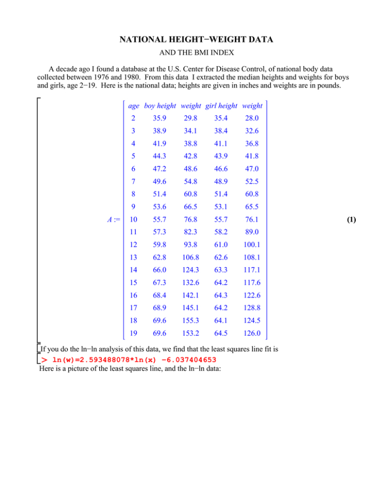
NATIONAL HEIGHT−WEIGHT DATA
AND THE BMI INDEX
A decade ago I found a database at the U.S. Center for Disease Control, of national body data
collected between 1976 and 1980. From this data I extracted the median heights and weights for boys
and girls, age 2−19. Here is the national data; heights are given in inches and weights are in pounds.
age boy height weight girl height weight
A :=
2
35.9
29.8
35.4
28.0
3
38.9
34.1
38.4
32.6
4
41.9
38.8
41.1
36.8
5
44.3
42.8
43.9
41.8
6
47.2
48.6
46.6
47.0
7
49.6
54.8
48.9
52.5
8
51.4
60.8
51.4
60.8
9
53.6
66.5
53.1
65.5
10
55.7
76.8
55.7
76.1
11
57.3
82.3
58.2
89.0
12
59.8
93.8
61.0
100.1
13
62.8
106.8
62.6
108.1
14
66.0
124.3
63.3
117.1
15
67.3
132.6
64.2
117.6
16
68.4
142.1
64.3
122.6
17
68.9
145.1
64.2
128.8
18
69.6
155.3
64.1
124.5
19
69.6
153.2
64.5
126.0
If you do the ln−ln analysis of this data, we find that the least squares line fit is
ln(w)=2.593488078*ln(x) −6.037404653
Here is a picture of the least squares line, and the ln−ln data:
(1)
national ln(ht)−ln(wt) data
5.5
5
4.5
4
3.5
3
2.5
3.2
3.4
3.6
3.8
4.0
4.2
4.4
x
You notice that until adolescence the boy and girl data are more or less indistinguishable. The "baby
fat" and big heads of small children may explain why the 2−year olds are slightly above the line, and the
peaking near adulthood for both the males and females is quite likely to be the effect of their respective
hormones. But this data IS very close to a linear fit. Is there any sort of biological advantage to this sort
of scaling?
Going back to the power law:
p:=2.593488078:
C:=exp(−6.037404653):
f:=x−>C*x^p:
And here’s a picture of the experimental power law, graphed with the actual heights and weights
National Power Law
160
140
120
100
80
60
40
20
0
0
10
20
30
40
50
60
70
x
Correlation coefficient: In statistics one measures for a possible linear relationship between variables
by using the sample correlation coefficient. In class notes we skipped, and in the text (page 197) there is
a discussion of the fact that the correlation coefficient is really the cosine of the angle between the
normalized vector of x−values and the normalized vector of y−values. (The normalization is to subtract
off the average values of each data set so that the averages are both zero.) A correlation coefficient near
1 implies high positive correlation. If you compute the correlation coefficient for our ln−ln data, using
several omitted steps and the definition for cos(theta):
dotprod x, y
costheta := x, y
norm x, 2 norm y, 2
costheta(xvect−xvectav,yvect−yvectav);
#this is the sample correlation coefficient for our
#ln−ln data.
0.9924868726
(2)
arccos(0.9924868726);
#the angle between our normalized deviation vectors,
#in radians
0.1226585027
(3)