MATH 5050/6815: Simulation extra credit problem: Last passage time
Last passage time
Definition 1: Lattice path. A path π from (1, 1) to (m, n) on N2 is an ordered collection
of integer sites
π = {v1 , v2 , ..., vk }
for some k ∈ N where v1 = (1, 1) and vk = (m, n). We call k the length of the path.
Definition 2: Directed lattice path. A directed lattice path π is a lattice path (as in
definition 1) so that
vj+1 − vj ∈ {(1, 0), (0, 1)}.
This means the path can take only horizontal steps form left to right and vertical steps
from south to north. The set of all directed lattice paths of length n, starting from (1, 1) is
denoted by Πn , while the set of all directed lattice path from (1, 1) to (k, `) is denoted by
Π(1,1),(k,`) .
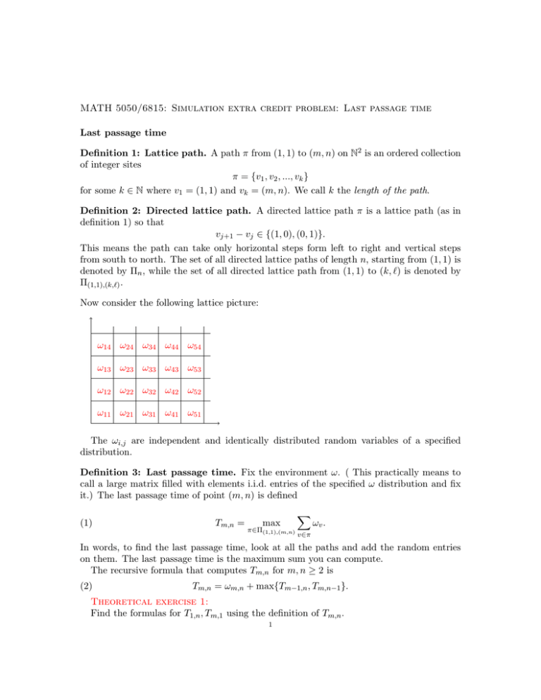
Now consider the following lattice picture:
ω14 ω24 ω34 ω44 ω54
ω13 ω23 ω33 ω43 ω53
ω12 ω22 ω32 ω42 ω52
ω11 ω21 ω31 ω41 ω51
The ωi,j are independent and identically distributed random variables of a specified
distribution.
Definition 3: Last passage time. Fix the environment ω. ( This practically means to
call a large matrix filled with elements i.i.d. entries of the specified ω distribution and fix
it.) The last passage time of point (m, n) is defined
(1)
Tm,n =
max
π∈Π(1,1),(m,n)
X
ωv .
v∈π
In words, to find the last passage time, look at all the paths and add the random entries
on them. The last passage time is the maximum sum you can compute.
The recursive formula that computes Tm,n for m, n ≥ 2 is
(2)
Tm,n = ωm,n + max{Tm−1,n , Tm,n−1 }.
Theoretical exercise 1:
Find the formulas for T1,n , Tm,1 using the definition of Tm,n .
1
2
Theoretical exercise 2:
Assume that E(ω1,1 ) = µ. Using your answer to the previous question and the law of
large numbers, find the limn→∞ n−1 T1,n , limm→∞ m−1 Tm,1 .
Simulation exercise 1:
Let N = 1500 and for x ∈ [0, 1] define
f (x) =
TbN xc,bN (1−x)c
.
N
Draw f (x) when:
(1) The distribution of ω is Bernoulli(p) for p = .1, .2, .5, .8, .9, .95. Observe anything
interesting?
(2) The distribution of ω is Exp(λ) for λ = 1.5, 2, 5, 8.
(3) The distribution of ω is N (0, σ 2 ) for σ = 1, 2.
(4) The distribution of ω is Uniform(a, b) for (a, b) = (0, 1), (−1, 1), (1, 2).
Simulation exercise 2.
Repeat the previous exercise for three other distributions for ω of your choice (not the
same as above). Also compare f (x) among the non negative distributions only. What are
the common properties?
Simulation exercise 3.
For each of the distributions in simulation exercise 1, compute V ar(TN,N ) using 500
samples for N = 1000 and N = 1500. (It’s going to take a while :)
Simulation exercise 4.
For each of the distributions in simulation exercise 1, plot the graph g(N ) = V ar(TN,N )
for 1 ≤ N ≤ 2000. Use 100 different samples to estimate each variance. After that plot
h(N ) = g(N/)N 2/3 .