MATH 5050/6815: Simulation extra credit problem: Random Polymers
Random Polymers in random environment.
Definition 1: Lattice path. A path π from (1, 1) to (m, n) on N2 is an ordered collection
of integer sites
π = {v1 , v2 , ..., vk }
for some k ∈ N where v1 = (1, 1) and vk = (m, n). We call k the length of the path.
Definition 2: Directed lattice path. A directed lattice path π is a lattice path (as in
definition 1) so that
vj+1 − vj ∈ {(1, 0), (0, 1)}.
This means the path can take only horizontal steps form left to right and vertical steps
from south to north. The set of all directed lattice paths of length n, starting from (1, 1) is
denoted by Πn , while the set of all directed lattice path from (1, 1) to (k, `) is denoted by
Π(1,1),(k,`) .
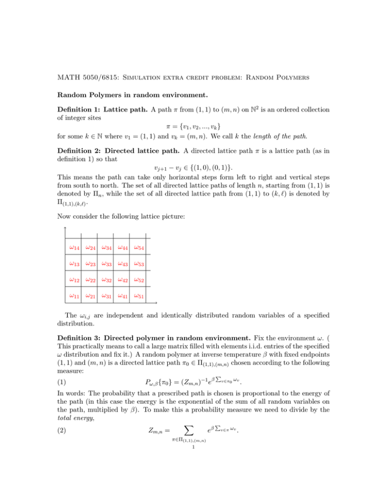
Now consider the following lattice picture:
ω14 ω24 ω34 ω44 ω54
ω13 ω23 ω33 ω43 ω53
ω12 ω22 ω32 ω42 ω52
ω11 ω21 ω31 ω41 ω51
The ωi,j are independent and identically distributed random variables of a specified
distribution.
Definition 3: Directed polymer in random environment. Fix the environment ω. (
This practically means to call a large matrix filled with elements i.i.d. entries of the specified
ω distribution and fix it.) A random polymer at inverse temperature β with fixed endpoints
(1, 1) and (m, n) is a directed lattice path π0 ∈ Π(1,1),(m,n) chosen according to the following
measure:
(1)
Pω,β {π0 } = (Zm,n )−1 e
β
P
v∈π0
ωv
.
In words: The probability that a prescribed path is chosen is proportional to the energy of
the path (in this case the energy is the exponential of the sum of all random variables on
the path, multiplied by β). To make this a probability measure we need to divide by the
total energy,
P
X
(2)
Zm,n =
eβ v∈π ωv .
π∈Π(1,1),(m,n)
1
2
The recursive formula that computes Zm,n for m, n ≥ 2 is
(3)
Zm,n = eβωm,n (Zm−1,n + Zm,n−1 ).
Theoretical exercise 1:
Find the formulas for Z1,n , Zm,1 using the definition of Zm,n .
Simulation exercise 1:
Let N = 1000, fix β = 1 and for x ∈ [0, 1] define
log ZbN xc,bN (1−x)c
f (x) =
.
N
Draw f (x) when:
(1) The distribution of ω is Bernoulli(p) for p = .1, .2, .5, .8, .9, .95. (One realization of
ω only).
(2) The distribution of ω is Exp(λ) for λ = 1.5, 2, 5, 8.
(3) The distribution of ω is N (0, σ 2 ) for σ = 1, 2.
(4) The distribution of ω is Uniform(a, b) for (a, b) = (0, 1), (−1, 1), (1, 2).
Simulation exercise 2.
Repeat the previous exercise for β = 0.1, 0.9, 1.5, 2, 10 and compare the functions across
β.
Simulation exercise 3.
For each of the distributions in simulation exercise 1, compute V ar(log ZN,N ) using 500
samples for N = 1000 and N = 1500. (It’s going to take a while :)
Simulation exercise 4.
For each of the distributions in simulation exercise 1, plot the graph g(N ) = V ar(log ZN,N )
for 1 ≤ N ≤ 2000. Use 100 different samples to estimate each variance. After that, plot
h(N ) = g(N )/N 2/3 .