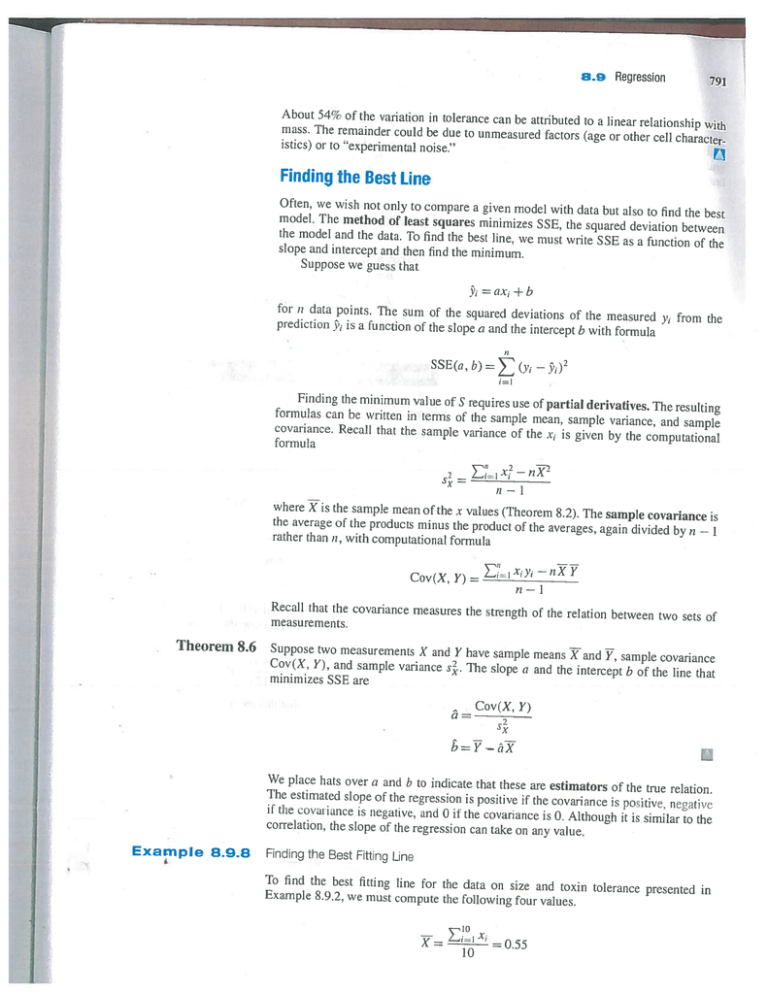
89 Regression
791
About 54% of the variation in tolerance can be attribu
ted to a linear relationship with
mass. The remainder could be due to unmeasured factors
(age or other cell character
istics) or to “experimental noise.”
fl
Finding the Best Line
Often, we wish not only to compare a given model with
data but also to find the best
model. The method of least squares minimizes SSE,
the squared deviation between
the model and the data. To find the best line, we must write
SSE as a function of the
slope and intercept and then find the minimum.
Suppose we guess that
—
ax + b
for ii data points. The sum of the squared deviations
of the measured y from the
prediction 5’ is a function of the slope a and the interce
pt b with formula
SSE(a, b)
(yi
=
—
5)2
Finding the minimum value of S requires use of parti
al derivatives. The resulting
formulas can be written in terms of the sample mean,
sample variance, and sample
covariance. Recall that the sample variance of the
x is given by the computational
formula
2
E
—
X
nX
—
u—i
where Xis the sample mean of the x values (Theorem 8.2).
The sample covariance is
the average of the products minus the product of the
averages, again divided by n 1
rather than n, with computational formula
—
Cov(X, Y)
xiyi
—
=
11
1
Recall that the covariance measures the strength of
the relation between two sets of
measurements.
—
Theorem 8.6
Suppose two measurements K and Y have sample means
Xand Y, sample covariance
Cov(X, Y), and sample variance s.. The slope a and
the intercept b of the line that
minimizes SSE are
a=
Cov(X, Y)
2
sx
We place hats over a and b to indicate that these are
estimators of the true relation.
The estimated slope of the regression is positive if
the covariance is positive, negative
if the covariance is negative, and 0 if the covariance
is 0. Although it is similar to the
correlation, the slope of the regression can take on any
value.
Example 8.9.8
Finding the Best FitUng Line
To find the best fitting line for the data on size and
toxin tolerance presented in
Example 8.9.2, we must compute the following four
values.
-=
>
10
=
0.55