Lecture 13
1. Inequalities
Let us start with an inequality.
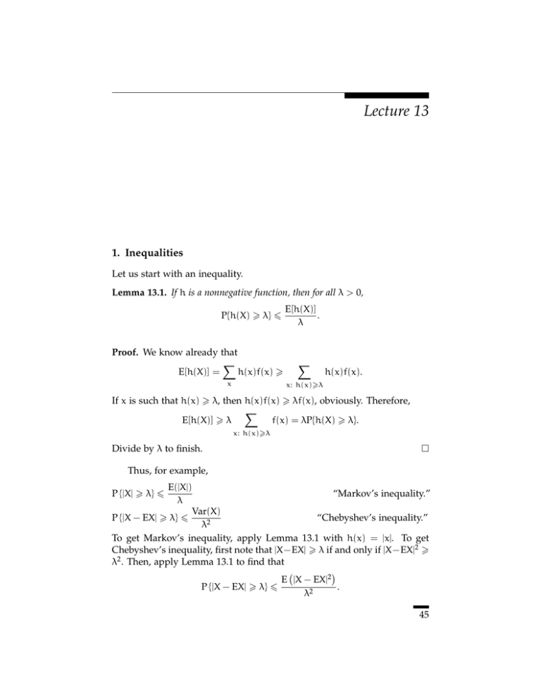
Lemma 13.1. If h is a nonnegative function, then for all λ > 0,
P{h(X) ! λ} "
Proof. We know already that
!
E[h(X)] =
h(x)f(x) !
x
E[h(X)]
.
λ
!
h(x)f(x).
x: h(x)!λ
If x is such that h(x) ! λ, then h(x)f(x) ! λf(x), obviously. Therefore,
!
E[h(X)] ! λ
f(x) = λP{h(X) ! λ}.
x: h(x)!λ
Divide by λ to finish.
#
Thus, for example,
E(|X|)
“Markov’s inequality.”
λ
Var(X)
P {|X − EX| ! λ} "
“Chebyshev’s inequality.”
λ2
To get Markov’s inequality, apply Lemma 13.1 with h(x) = |x|. To get
Chebyshev’s inequality, first note that |X−EX| ! λ if and only if |X−EX|2 !
λ2 . Then, apply Lemma 13.1 to find that
!
"
E |X − EX|2
P {|X − EX| ! λ} "
.
λ2
P {|X| ! λ} "
45
46
13
Then, recall that the numerator is Var(X).
In words:
• If E(|X|) < ∞, then the probability that |X| is large is small.
• If Var(X) is small, then with high probability X ≈ EX.
2. Conditional distributions
If X is a random variable with mass function f, then {X = x} is an event.
Therefore, if B is also an event, and if P(B) > 0, then
P(X = x | B) =
P({X = x} ∩ B)
.
P(B)
As we vary the variable x, we note that {X = x} ∩ B are disjoint. Therefore,
#
!
P({X = x} ∩ B)
P (∪x {X = x} ∩ B)
P(X = x | B) =
=
= 1.
P(B)
P(B)
x
Thus,
f(x | B) = P(X = x | B)
defines a mass function also. This is called the conditional mass function of
X given B.
Example 13.2. Let X be distributed uniformly on {1 , . . . , n}, where n is a
fixed positive integer. Recall that this means that

1
if x = 1, . . . , n,
f(x) = n
0 otherwise.
Choose and fix two integers a and b such that 1 " a " b " n. Then,
P{a " X " b} =
b
!
1
b−a+1
=
.
n
n
x=a
Therefore,
f(x | a " X " b) =


1
b−a+1
0
if x = a, . . . , b,
otherwise.
47
3. Conditional expectations
3. Conditional expectations
Once we have a (conditional) mass function, we have also a conditional
expectation at no cost. Thus,
!
E(X | B) =
xf(x | B).
x
Example 13.3 (Example 13.2, continued). In Example 13.2,
E(X | a " X " b) =
b
!
k=a
Now,
b
!
k=
k=a
b
!
k=1
k−
a−1
!
k
.
b−a+1
k
k=1
b(b + 1) (a − 1)a
=
−
2
2
b2 + b − a2 + a
=
.
2
Write b2 − a2 = (b − a)(b + a) and factor b + a to get
b
!
k=a
Therefore,
k=
b+a
(b − a + 1).
2
b+a
.
2
This should not come as a surprise. Example 13.2 actually shows that
given B = {a " X " b}, the conditional distribution of X given B is uniform
on {a, . . . , b}. Therefore, the conditional expectation is the expectation of a
uniform random variable on {a, . . . , b}.
E(X | a " X " b) =
Theorem 13.4 (Bayes’s formula for conditional expectations). If P(B) > 0,
then
EX = E(X | B)P(B) + E(X | Bc )P(Bc ).
Proof. We know from the ordinary Bayes’s formula that
f(x) = f(x | B)P(B) + f(x | Bc )P(Bc ).
Multiply both sides by x and add over all x to finish.
#
48
13
Remark 13.5. The more general version of Bayes’s formula works too here:
Suppose B1 , B2 , . . . are disjoint and ∪∞
i=1 Bi = Ω; i.e., “one of the Bi ’s happens.” Then,
∞
!
EX =
E(X | Bi )P(Bi ).
i=1
Example 13.6. Suppose you play a fair game repeatedly. At time 0, before
you start playing the game, your fortune is zero. In each play, you win
or lose with probability 1/2. Let T1 be the first time your fortune becomes
+1. Compute E(T1 ).
More generally, let Tx denote the first time to win x dollars, where
T0 = 0.
Let W denote the event that you win the first round. Then, P(W) =
P(W c ) = 1/2, and so
1
1
E(Tx ) = E(Tx | W) + E(Tx | W c ).
(11)
2
2
Suppose x $= 0. Given W, Tx is one plus the first time to make x − 1 more
dollars. Given W c , Tx is one plus the first time to make x + 1 more dollars.
Therefore,
$ 1#
$
1#
E(Tx ) = 1 + E(Tx−1 ) + 1 + E(Tx+1 )
2
2
E(Tx−1 ) + E(Tx+1 )
=1+
.
2
Also E(T0 ) = 0.
Let g(x) = E(Tx ). This shows that g(0) = 0 and
g(x + 1) + g(x − 1)
2
Because g(x) = (g(x) + g(x))/2,
g(x) = 1 +
g(x) + g(x) = 2 + g(x + 1) + g(x − 1)
Solve to find that for all integers x ! 1,
for x = ±1, ±2, . . . .
for x = ±1, ±2, . . . .
g(x + 1) − g(x) = −2 + g(x) − g(x − 1).