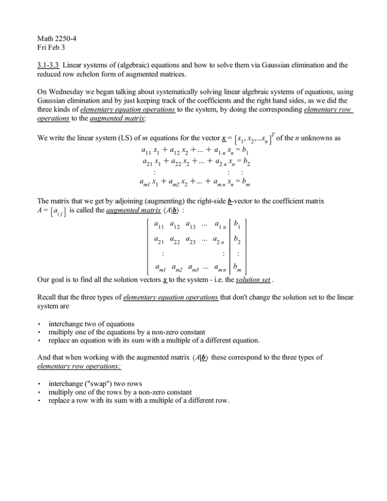
Math 2250-4
Fri Feb 3
3.1-3.3 Linear systems of (algebraic) equations and how to solve them via Gaussian elimination and the
reduced row echelon form of augmented matrices.
On Wednesday we began talking about systematically solving linear algebraic systems of equations, using
Gaussian elimination and by just keeping track of the coefficients and the right hand sides, as we did the
three kinds of elementary equation operations to the system, by doing the corresponding elementary row
operations to the augmented matrix:
We write the linear system (LS) of m equations for the vector x = x1 , x2 ,...xn
a11 x1 C a12 x2 C... C a1 n xn = b1
a21 x1 C a22 x2 C... C a2 n xn = b2
:
: :
am1 x1 C am2 x2 C... C am n xn = bm
T
of the n unknowns as
The matrix that we get by adjoining (augmenting) the right-side b-vector to the coefficient matrix
A = ai j is called the augmented matrix A b :
a11 a12 a13 ...
a1 n
b1
a21 a22 a23 ... a2 n
b2
:
:
:
am1 am2 am3 ... am n bm
Our goal is to find all the solution vectors x to the system - i.e. the solution set .
Recall that the three types of elementary equation operations that don't change the solution set to the linear
system are
,
,
,
interchange two of equations
multiply one of the equations by a non-zero constant
replace an equation with its sum with a multiple of a different equation.
And that when working with the augmented matrix A b these correspond to the three types of
elementary row operations:
,
,
,
interchange ("swap") two rows
multiply one of the rows by a non-zero constant
replace a row with its sum with a multiple of a different row.
Exercise 1: Use Gaussian elimination on the augmented matrices to finish the example systems from
Wednesday notes. Each of these is a system of three equations in three unknowns, so can be interpreted as
looking for the intersection set of three planes in =3 (even though the system may have arisen in a
completely different context). Even though the systems are nearly identical, we'll get a different type of
solution set each time!
1a)
xC2 yCz = 4
3 x C 8 y C 7 z = 20
2 x C 7 y C 9 z = 23 .
(Hint: the solution set is a single point x, y, z = 5,K2, 3 ).
1b)
xC2 yCz = 4
3 x C 8 y C 7 z = 20
2 x C 7 y C 8 z = 20 .
Hint: the solution set is a line in =3 !
1c)
xC2 yCz = 4
3 x C 8 y C 7 z = 20
2 x C 7 y C 8 z = 23 .
Hint: the solution set is empty !
1d) What are the possible solution sets (and geometric configurations) for 1, 2, 3, 4,... equations in 3
unknowns?
Let's do a bigger example, to carefully illstrate the Gaussian elimination algorithm we've been using for
finding the solution set to any linear system of equations. We will use elementary row operations and
work column by column (from left to right) and row by row (from top to bottom) to first get the
augmented matrix for an equivalent system of equations which is in
row-echelon form:
(1) All "zero" rows (having all entries = 0) lie beneath the non-zero rows.
(2) The leading (first) non-zero entry in each non-zero row lies strictly to the right of the one above
it.
(At this stage you could "backsolve" to find all solutions.)
Continue with Gaussian elimination, but working from bottom to top and from right to left so that we end
with an augmented matrix that is in
reduced row echelon form: (1),(2), together with
(3) Each leading non-zero row entry has value 1 . Such entries are called "leading 1's "
(4) Each column that has (a row's) leading 1 has 0's in all the other entries.
Finally, read off how to explicitly specify the solution set.
Note: There are lots of row-echelon forms for a matrix, but only one reduced row-echelon form. All
mathematical software will have a command to find the reduced row echelon form.
Here's our system...
x1 K 2 x2 C 3 x3 C 2 x4 C x5 = 10
2 x1 K 4 x2 C 8 x3 C 3 x4 C 10 x5 = 7
3 x1 K 6 x2 C 10 x3 C 6 x4 C 5 x5 = 27 .
Exercise 2: The augmented matrix for the system above is
1 K2
3 2
1 10
2 K4
8 3 10
7
3 K6 10 6 5 27
Find the reduced row echelon form of this augmented matrix and then backsolve to explicitly parameterize
the solution set. (Hint: it's a three-dimensional plane in =5 , if that helps. :-) )
Maple says:
> with LinearAlgebra : # matrix and linear algebra library
> A d Matrix 3, 5, 1,K2, 3, 2, 1,
2,K4, 8, 3, 10,
3,K6, 10, 6, 5 :
b d Vector 10, 7, 27 :
A b ; # the mathematical augmented matrix doesn't actually have
# a vertical line between the end of A and the start of b
ReducedRowEchelonForm A b ;
1 K2
3 2
1 10
2 K4
8 3 10
7
3 K6 10 6
5 27
1 K2 0 0
3
0
0 1 0
2 K3
0
0 0 1 K4
5
7
> LinearSolve A, b :
# this command will actually write down the general solution, using
# Maple's way of writing free parameters, which actually makes
# some sense. Generally when there are free parameters involved,
# there will be equivalent ways to express the solution that may
# look different. But usually Maple's version will look like yours.
>
(1)