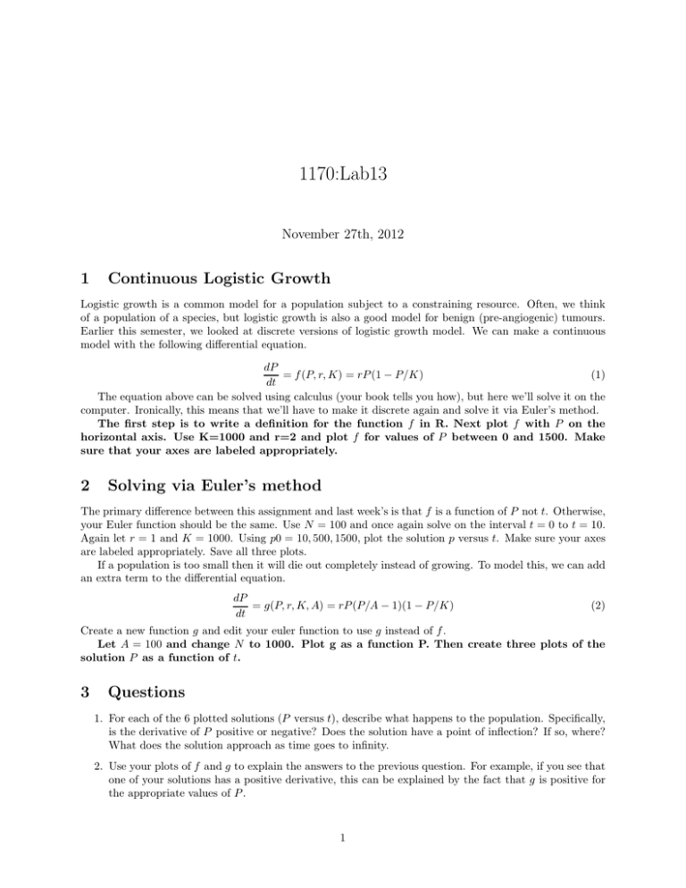
1170:Lab13
November 27th, 2012
1
Continuous Logistic Growth
Logistic growth is a common model for a population subject to a constraining resource. Often, we think
of a population of a species, but logistic growth is also a good model for benign (pre-angiogenic) tumours.
Earlier this semester, we looked at discrete versions of logistic growth model. We can make a continuous
model with the following differential equation.
dP
= f (P, r, K) = rP (1 − P/K)
(1)
dt
The equation above can be solved using calculus (your book tells you how), but here we’ll solve it on the
computer. Ironically, this means that we’ll have to make it discrete again and solve it via Euler’s method.
The first step is to write a definition for the function f in R. Next plot f with P on the
horizontal axis. Use K=1000 and r=2 and plot f for values of P between 0 and 1500. Make
sure that your axes are labeled appropriately.
2
Solving via Euler’s method
The primary difference between this assignment and last week’s is that f is a function of P not t. Otherwise,
your Euler function should be the same. Use N = 100 and once again solve on the interval t = 0 to t = 10.
Again let r = 1 and K = 1000. Using p0 = 10, 500, 1500, plot the solution p versus t. Make sure your axes
are labeled appropriately. Save all three plots.
If a population is too small then it will die out completely instead of growing. To model this, we can add
an extra term to the differential equation.
dP
= g(P, r, K, A) = rP (P/A − 1)(1 − P/K)
dt
(2)
Create a new function g and edit your euler function to use g instead of f .
Let A = 100 and change N to 1000. Plot g as a function P. Then create three plots of the
solution P as a function of t.
3
Questions
1. For each of the 6 plotted solutions (P versus t), describe what happens to the population. Specifically,
is the derivative of P positive or negative? Does the solution have a point of inflection? If so, where?
What does the solution approach as time goes to infinity.
2. Use your plots of f and g to explain the answers to the previous question. For example, if you see that
one of your solutions has a positive derivative, this can be explained by the fact that g is positive for
the appropriate values of P .
1