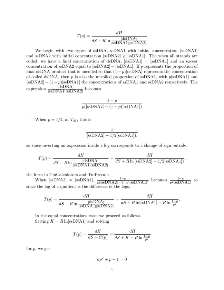
T (p) =
dH
[dsDNA]
dS − R ln [ssDNA1
][ssDNA2]
We begin with two types of ssDNA, ssDNA1 with initial concentration [ssDNA1]
and ssDNA2 with initial concentration [ssDNA2] ≥ [ssDNA1]. The when all strands are
coiled, we have a final concentration of dsDNA, [dsDNA1] = [ssDNA1] and an excess
concentration of ssDNA2 equal to [ssDNA2] − [ssDNA1]. If p represents the proportion of
final dsDNA product that is uncoiled so that (1 − p)[dsDNA] represents the concentration
of coiled dsDNA, then p is also the uncoiled proportion of ssDNA1, with p[ssDNA1] and
[ssDNA2] − (1 − p)[ssDNA1] the concentrations of ssDNA1 and ssDNA2 respectively. The
[dsDNA]
expression
becomes
[ssDNA1][ssDNA2]
1−p
p([ssDNA2] − (1 − p)[ssDNA1])
.
When p = 1/2, at TM , this is
1
[ssDNA2] − 1/2[ssDNA1]).
so since inverting an expression inside a log corresponds to a change of sign outside,
T (p) =
dH
dH
,
=
[dsDNA]
dS
+
R
ln
[ssDNA2]
−
1/2[ssDNA1])
dS − R ln
[ssDNA1][ssDNA2]
the form in TmCalculators and TmPrecalc.
1−p
When [ssDNA2] = [ssDNA1], p([ssDNA2]−(1−p)[
ssDNA1]) becomes
since the log of a quotient is the difference of the logs,
T (p) =
1−p
p2 [ssDNA1]
dH
dH
=
.
[dsDNA]
dS + R ln[ssDNA1] − R ln 1−p
dS − R ln [ssDNA1
p2
][ssDNA2]
In the equal concentrations case, we proceed as follows.
Setting K = R ln[ssDNA1] and solving
T (p) =
dH
dH
=
dS + C(p)
dS + K − R ln 1−p
p2
for p, we get
ap2 + p − 1 = 0
1
so
Here p is the proportion uncoiled and 1 − p is the proportion coiled, and a = e−dG(T ) ,
where G = (dH − T dS − KT )/RT , where K depends only on probe and target concentrations, and dH and dS depend only upon the nearest neighbor parameters and properties
of the oligo under consideration.
Since we know C(.5), we can obtain
K = C(.5) + R ln .5.
Dividing by a and setting v = 1/a, we solve for the positive root p of the quadratic
equation
p2 + vp − v = 0,
√
v 2 + 4v
.
2
Some observations about the dependence of G, a, and v on T .
Since dH < 0, dS < 0, K < 0 (depending upon [ssDNA1]), as T → 0, dG = (dH −
dH −dS−K
=→ −∞ so a → +∞, v → 0+ .
T dS − KT )/RT = ( RT
R
Interestingly, as T → +∞, dG → −dS−K
> 0, a → a∗ with 0 < a∗ << 1, v → v∗ with
R
1 << v∗ << +∞.
So as T → 0, p → 0 and the fraction coiled 1 − p → 1. but as T → +∞, p → p∗ with
0 < 1 − p∗ << 1. A minimum proportion of DNA remains coiled no matter how great T
becomes.
Rewriting
√
−v + v 2 + 4v
p=
2
in terms of w = v + 2 to complete the square, we obtain
p
−(v + 2) + 2 + (v + 2)2 − 4
p=
2
p=
−v +
or
p=1−
w−
√
w2 − 4
2
from which the fraction coiled, 1 − p becomes
w
1−p= −
2
r
w2
−1
2
)
= 1+ 12 edG(T ) . So w → 1 as T → 0. The melting temperature TM is where
where w2 = w(T
2
√
this difference is 1/2. Solving x − 1/2 = x2 − 1, we get this occurs when x = w/2 = 5/4.
So the sharp phase transition is due to the fact that edG(T ) remains very small until
the melting temperature then grows quickly to its large positive limit edG∗ . edG(T ) is of
b
the form ea− T , where a > 0, b > 0, so when T is small, the second term is dominant and
the result is extremely small, but as T grows, the first term eventually dominates, with
2
a rapid transition to extremely large values. This function becomes the argument of a
function with values near 1 for small values of its argument, and near zero for large values
of its argument, hence the form of the melting curves.
In the general case,
T (p) =
dH
dH
=
1−p
[dsDNA]
dS − R ln p([ssDNA2]−(1−p)[
dS − R ln [ssDNA1
ssDNA1])
][ssDNA2]
.
Rearranging again,
p([ssDNA2] − (1 − p)[ssDNA1])e−
[ssDNA1])e−
dH−T dS
RT
dH−T dS
RT
+p−1= 0
p2 + (1 + ([ssDNA2] − [ssDNA1])e−
dH−T dS
RT
)−1=0
ap2 + bp − 1 = 0
dH−T dS
dH−T dS
where a = [ssDNA1]e− RT
and b = 1 + ([ssDNA2] − [ssDNA1])e− RT )
We note that when the initial concentrations are equal, the general case reduces to the
original equal concentration case, since the expression for b becomes 1, and the expression
for a is identical to the expression for a only depends on the smaller initial concentration.
Also, since the equal concentration case K = R ln[ssDNA1] a may also be written as
dH−T dS−KT
RT
, no different than in the equal concentration case, and in that case,
e−
If we let d = [ssDNA2] − [ssDNA1] so that b = 1 + d, and again dividing through by
− a1 = 0, we call v = a1 (which has
a, so the quadratic equation becomes monic, p2 + (1+d)
a
the same value as before in terms of the initial concentration of ssDNA1 and dH, dS, and
R so p2 + (1 + d)vp − v = 0 and the melting curve solution is given by
p
−(1 + d)v + ((1 + d)v)2 + 4v
p=
.
2
Exercise: Complete the square and try to make analogous transformations to obtain
a simpler form for 1 − p as in the equal concentration case.
3
In the equal concentrations case, we are able to compute T (p) for different p by
, and either using the formula K = R ln[ssDNA1] or
determining C(p) = K − R ln 1−p
p2
solving for K from the known value of C(p) when p = .5, C(.5)=R ln[ssDNA1] C(.5) =
2
so we only
K − ln 2, so K = C(.5) + ln 2. Another form is C(p) = C(.5) + ln 2 − R ln 1−p
p2
need to know C(.5) the factor used in the melting temperature calculator to compute all
other T (p)s.
This is not so in the general case. To compute C(p), hence T (p), use
T (p) =
.
dH
dH
=
1−p
[dsDNA]
dS − R ln p([ssDNA2]−(1−p)[
dS − R ln
ssDNA1])
[ssDNA1][ssDNA2]
1−p
Here, C(.5) = −R ln p([ssDNA2]−(1−p)[
ssDNA1]) = R ln([ssDNA2] − .5[ssDNA1]) is
not enough to compute C(p).
Note that p([ssDNA2]−(1−p)[ssDNA1]) may be rewritten p2 [ssDNA1]+p([ssDNA2]−
[ssDNA1])
TmCalculators and TmPrecalculators computed C(.5) and for the equal concentration
first example, we did use this to compute other TM s for parameter inversion. To do
this in more generality, “T (p)-Precalc” must provide the data necessary to compute the
coefficients for melting curve inversion and computing the temperature for an arbitrary
fraction uncoiled, p. so TpPrecalc.vi delivers [ssDNA1] and [ssDNA2] − [ssDNA1] along
with the salt dependent length factor.
T (p)-calculator takes these values and given p, as well as the values of dH and dS
and the length of the oligo, computes T (p). The default is p = .5, which reduces to a TM
calculator.
Curve.vi takes values of dH, dS and the length of an oligo, combines them with the
initial concentrations and salt factor from T(p)-precalc, and for any value of T , computes
the coefficients of the quadratic and solves them for p(T ).
4