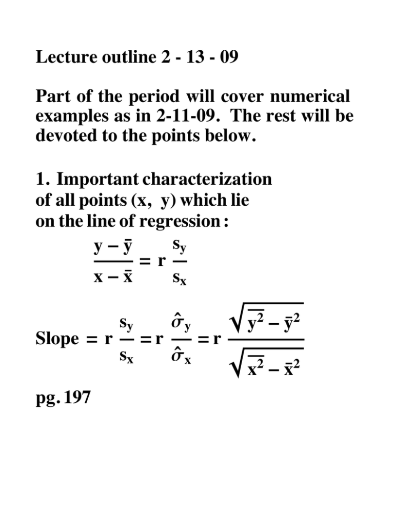
Lecture outline 2 - 13 - 09
Part of the period will cover numerical
examples as in 2-11-09. The rest will be
devoted to the points below.
1. Important characterization
of all points Hx, yL which lie
on the line of regression :
sy
y-y
=r
x-x
sx
`
sy
sy
Slope = r = r ` = r
sx
sx
pg. 197
y2 - y2
x2 - x2
2
Lecture Outline 2-13-09.nb
2. Taking x = 0 in
y-y
0-x
= r
sy
sx
gives
intercept = y - x slope
pg. 198
3. For every x, solving for y in
sy
y-y
= r
x-x
sx
gives predicted y = pt on regr line :
pred y = y + Hx - xL slope
Lecture Outline 2-13-09.nb
4. For an approximately
ELLIPTICAL plot, at a given x
the distribution of y is approximately
NORMAL with
mean = predicted y
std dev = 1 - r2 sy
Notice that the mean depends
upon x but the std dev does not.
5. For an ELLIPTICAL PLOT
the regression predictor
y + Hx - xL slope
is optimal in the sense of least
mean squared error of prediction.
` 2
5. r is exactly the fraction of s y
explained by the sample regression.
2
3
4
Lecture Outline 2-13-09.nb
` 2
5. r is exactly the fraction of s y
explained by the sample regression.
2
pp. 204-06 (Note text also uses R for r.
The Greek "rho" r is also used for r).