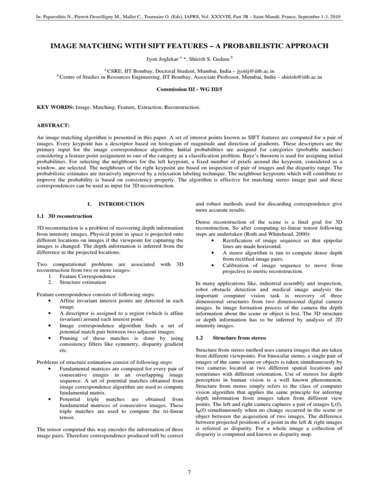
In: Paparoditis N., Pierrot-Deseilligny M., Mallet C., Tournaire O. (Eds), IAPRS, Vol. XXXVIII, Part 3B – Saint-Mandé, France, September 1-3, 2010
IMAGE MATCHING WITH SIFT FEATURES – A PROBABILISTIC APPROACH
Jyoti Joglekar a, *, Shirish S. Gedam b
b
a
CSRE, IIT Bombay, Doctoral Student, Mumbai, India – jyotij@iitb.ac.in
Centre of Studies in Resources Engineering, IIT Bombay, Associate Professor, Mumbai, India – shirish@iitb.ac.in
Commission III - WG III/5
KEY WORDS: Image, Matching, Feature, Extraction, Reconstruction.
ABSTRACT:
An image matching algorithm is presented in this paper. A set of interest points known as SIFT features are computed for a pair of
images. Every keypoint has a descriptor based on histogram of magnitude and direction of gradients. These descriptors are the
primary input for the image correspondence algorithm. Initial probabilities are assigned for categories (probable matches)
considering a feature point assignment to one of the category as a classification problem. Baye’s theorem is used for assigning initial
probabilities. For selecting the neighbours for the left keypoint, a fixed number of pixels around the keypoint, considered as a
window, are selected. The neighbours of the right keypoint are based on inspection of pair of images and the disparity range. The
probabilistic estimates are iteratively improved by a relaxation labeling technique. The neighbour keypoints which will contribute to
improve the probability is based on consistency property. The algorithm is effective for matching stereo image pair and these
correspondences can be used as input for 3D reconstruction.
1.
and robust methods used for discarding correspondence give
more accurate results.
INTRODUCTION
1.1 3D reconstruction
Dense reconstruction of the scene is a final goal for 3D
reconstruction. So after computing tri-linear tensor following
steps are undertaken (Roth and Whitehead, 2000):
•
Rectification of image sequence so that epipolar
lines are made horizontal.
•
A stereo algorithm is run to compute dense depth
from rectified image pairs.
•
Calibration of image sequence to move from
projective to metric reconstruction.
3D reconstruction is a problem of recovering depth information
from intensity images. Physical point in space is projected onto
different locations on images if the viewpoint for capturing the
images is changed. The depth information is inferred from the
difference in the projected locations.
Two computational problems are associated
reconstruction from two or more images:
1. Feature Correspondence
2. Structure estimation
with
3D
In many applications like, industrial assembly and inspection,
robot obstacle detection and medical image analysis the
important computer vision task is recovery of three
dimensional structures from two dimensional digital camera
images. In image formation process of the camera the depth
information about the scene or object is lost. The 3D structure
or depth information has to be inferred by analysis of 2D
intensity images.
Feature correspondence consists of following steps:
•
Affine invariant interest points are detected in each
image.
•
A descriptor is assigned to a region (which is affine
invariant) around each interest point.
•
Image correspondence algorithm finds a set of
potential match pair between two adjacent images.
•
Pruning of these matches is done by using
consistency filters like symmetry, disparity gradient
etc.
1.2
Structure from stereo
Structure from stereo method uses camera images that are taken
from different viewpoints. For binocular stereo, a single pair of
images of the same scene or objects is taken simultaneously by
two cameras located at two different spatial locations and
sometimes with different orientation. Use of stereos for depth
perception in human vision is a well known phenomenon.
Structure from stereo simply refers to the class of computer
vision algorithm that applies the same principle for inferring
depth information from images taken from different view
points. The left and right camera captures a pair of images IL(f),
IR(f) simultaneously when no change occurred in the scene or
object between the acquisition of two images. The difference
between projected positions of a point in the left & right images
is referred as disparity. For a whole image a collection of
disparity is computed and known as disparity map.
Problems of structure estimation consist of following steps:
•
Fundamental matrices are computed for every pair of
consecutive images in an overlapping image
sequence. A set of potential matches obtained from
image correspondence algorithm are used to compute
fundamental matrix.
•
Potential triple matches are obtained from
fundamental matrices of consecutive images. These
triple matches are used to compute the tri-linear
tensor.
The tensor computed this way encodes the information of three
image pairs. Therefore correspondence produced will be correct
7
In: Paparoditis N., Pierrot-Deseilligny M., Mallet C., Tournaire O. (Eds), IAPRS, Vol. XXXVIII, Part 3B – Saint-Mandé, France, September 1-3, 2010
The feature correspondence problem can be best explained by
an example. For instance a physical 3D point is projected on to
Image X as point 1 and image Y as point 2. Then point 1 and
point 2 are said to be correspondences. Hence the feature
correspondence or feature matching problem is to find the point
2 on image Y given the location of point 1 on image X. Human
vision is superb in solving this problem. Solving the problem
by automation of process by computers is rather difficult. It
searches the whole image Y for a point on image X. Some
constraints can narrow down the search, but if sufficient
constraints are not there the problem becomes difficult.
presented in (Mikolajczyk and Schmid, 2004). It is known as
gradient location and orientation histogram (GLOH). As
number of directions chosen to represent the histogram in
GLOH are more than SIFT the size of the descriptor is large in
GLOH descriptor. The size is reduced using principle
component analysis.
Nowadays many detectors and descriptors algorithms are
available for detecting corners edges and regions of interest. A
vector is associated with it as a descriptor. The SIFT algorithm
by Lowe is explained here which is used to provide primary
input to the image matching algorithm explained in section 3.
The detected region should have a shape which is a function of
the image. To characterize the region invariant descriptor is
computed for the extracted region.
The second problem of structure estimation is relatively easy in
comparison. After solving the correspondence problem a set of
points are computed. If intrinsic and extrinsic parameters of the
camera are known then exact reconstruction in absolute coordinates is possible. However the accuracy of the
reconstruction depends on accuracy of these parameters. In
addition, any errors in solving the correspondence problem
between two images also affect the accuracy of the
reconstruction. So, even if intrinsic and extrinsic parameters are
known, the challenge remains for developing the matching
algorithm that reduces the errors in the preprocessing steps to
estimate the structure.
For computing SIFT features and assigning descriptors to the
features following procedure is used. : A pyramid of images is
constructed with different scales of Gaussian function. From
these Gaussian smoothed images Difference of Gaussian
images are computed at different scales. Difference of Gaussian
function detects the interest points invariant to scale and
orientation in scale-space. The Difference of Gaussian function
will have strong response along edges, though the location
along the edge is poorly determined, as these locations are
unstable to small amount of noise. A poorly defined peak in the
Difference of Gaussian function will have a large principle
curvature across the edge but small along perpendicular
direction. Over all scales image locations are found to detect
the extrema. Scales of keypoint is used to select the Gaussian
smoothed image of closest scale, so that the computations are
performed in scale invariant manner.
2. DETECTOR AND DESCRIPTOR
2.1
Point Detectors and Descriptors
Parts of the image that have special properties and have some
structural significance are usually referred as image features.
The regions having visually identifiable textures are also
referred as image features. Some of the examples are edges,
corners, image gradients etc. Many computer vision
applications have feature extraction process as an intermediate
step for locating particular elements on an image. While
extracting features some of the important factors to be
considered are invariance, detectability, interpretability and
accuracy. Many applications in the area of photogrammetry and
computer vision use feature extraction as primary input for
further processing and analysis. Features are used for image
registration, 3D reconstruction, motion tracking etc. Invariance
property of feature extractor is very important as under
different transformations (geometric and radiometric) the same
features should be detectable in pair of stereo images, so that
they will be useful for matching process. (Remondino, 2006)
For keypoint localization a model based on Taylor series is fit
to every keypoint location and scale. Here stability (i.e.
invariance to transformation) is the measure of selecting the
interest points. For each image sample for the scale L, gradient
magnitude and orientation is computed using pixel difference.
Considering image gradient at every keypoint one or more
orientations are assigned to the keypoints. These orientations
and the respective magnitude at selected scales are used to
construct a 3D histogram for the region around the keypoint.
The descriptor computed using these gradient magnitude and
orientation at each image sample point is weighted by Gaussian
window. A Gaussian weighting function with σ equal to one
half of the width of the descriptor window is used to assign a
weight to the magnitude of each sample point. This Scale
invariant feature descriptor for every keypoint is of dimension
128 (Lowe, 2004).
2D locations in the images are located by the detectors. After
analyzing the region around the location a descriptor is
assigned to the location (interest point) which characterizes the
interest point under consideration with respect to its
neighboring points, using information about neighboring points
like intensity variation, change in gradient, histogram
considering gradient direction and magnitude.
2.2
3. MATCHING MODEL
When the set of keypoints are found next step is to construct a
set of possible matches. Ideally we want to match each
keypoint in the left image, which is considered as reference
image, with a keypoint in the right image. But in reality in a
stereo image pair we can find valid matches for some of the
keypoints in the left image.
SIFT Algorithm
In SIFT descriptor (Lowe, 2004) DoG detector is used to detect
interest points and the extracted regions are described by a
vector of dimension 128. The descriptor is normalized by
dividing the descriptor vector by square root of sum of the
squared components, so that the descriptor becomes
illumination invariant. A 3D histogram of gradient location and
orientation is used as a descriptor. With various measures it is
demonstrated that SIFT descriptors outperform (Mikolajczyk
and Schmid, 2003). Extended version of SIFT descriptor was
A primary input to the matching algorithm is a set of keypoint
with their descriptors computed using SIFT algorithm,
explained in the section 2.2.
An image correspondence algorithm is proposed and presented
in detail steps as below.
8
In: Paparoditis N., Pierrot-Deseilligny M., Mallet C., Tournaire O. (Eds), IAPRS, Vol. XXXVIII, Part 3B – Saint-Mandé, France, September 1-3, 2010
1.
2.
3.
4.
5.
6.
7.
8.
9.
10.
11.
16.
Key-points selection in both the images (left and
right) with SIFT.
For every keypoint from both the images a
descriptor is computed as below
i)
Around every keypoint a pixel area of size
16 x 16 is considered.
ii)
For each sample of size 4 x 4 gradient
magnitude & orientation are assigned.
iii)
A histogram of Gradient orientation
showing 8 bins gives a descriptor for every
4 x 4 sample size.
iv)
For a 16 x 16 sample size around the
keypoint a descriptor vector of dimension
4 x 4 x 8 is obtained.
An approximate maximum disparity range is
found by visual inspection of few matching
keypoints in the stereo image pair. The disparity
is present in the left and right image as the
stereo images are captured from different
viewpoints and orientations.
An area is selected around every right keypoint
node, considering possible maximum disparity
range.
All the keypoints are found in the area selected
in step 4, around a right keypoint node in the
right image.
The procedure of step 4 and 5 is iteratively
performed for all the right keypoints and the
area around each right keypoint is selected
considering the approximate maximum disparity
range.
The procedure in steps 4 and 5 is repeated for all
left keypoints from left image iteratively. But
here area around the left keypoint is a fixed
sample area of size 16 x 16
As shown in figure 1, the left keypoint node bi
is paired with every right keypoint node ci and
the pair is called as category pair
For every category pair, Euclidian distance
between the descriptors of the keypoints is
calculated.
Weight is assigned to every right keypoint ci , in
the selected area. The weight is inversely
proportional to the Euclidian distance between
the corresponding descriptors.
For every category ci the weight is calculated as
17.
p io (c ) = 1 − max ( wi (c))
c≠c
18.
12.
13.
14.
15.
1
, c≠c
k × ε i (c ) + 1
(2)
By applying Baye’s rule
p io (c ) = p i (c i) × (1 − p io (c )) , c ≠ c
p i (c i )
:
(3)
conditional probability that bi has
category c as matching, given
that bi is matchable
(1 − p io (c ) ) : prior probability that bi
matchable
19.
is
Estimating p i (c i ) as below
p i (c i ) =
wi (c)
L
(4)
∑ wi (c ′)
c '=1
c '≠ c
20.
21.
22.
wi (c ) =
The weights can not be used as probability
estimates as wi (c ) is undefined and weights
will not sum up to 1.
Considering the keypoint matching as a
classification problem, bi is classified to one of
the category ci. Initial probability for undefined
category is given as
(1)
23.
k is a positive constant
A disparity category which associates highly
similar pairs of region will have large weight
value.
wi (c) will be in the interval [0, 1] and weight is
inversely proportional to Euclidian distance.
For every category set c, c is undefined
disparity category.
Consider weight wi (c ) for c which is
undefined i.e. keypoint bi(x,y) from left image
does not correspond to any keypoint in the right
selection area of right image.
Initial probabilities are assigned to every
category ci from right selection by equation (2),
(3) and (4).
Initial probabilities which depend only on the
similarity of neighborhood of candidate
matching points can be improved using
consistency property.
The probability updating rule should have
following property :
The new probability pik +1 (c) should tend to
increase when descriptors with highly probable
category consistent with c are found nearby the
keypoint region.
Categories are considered consistent if they
represent nearly the same disparity i.e.
d (ci ) − d (cm ) < Threshold: The threshold has
to be decided empirically by inspection of stereo
image pair.
24.
9
For computing new probability pik +1 (c) for all
ci in category set c, likelihood estimation is
done.
The degree to which the cj of c strengthen pi(c)
should be related to estimated likelihood.
In: Paparoditis N., Pierrot-Deseilligny M., Mallet C., Tournaire O. (Eds), IAPRS, Vol. XXXVIII, Part 3B – Saint-Mandé, France, September 1-3, 2010
qijk (c) =
Figure 2 is a test stereo image pair. Figure 3 shows the
performance of the algorithm using Euclidian distance and Best
Bin First approach to compare closest neighbor to that of
second closest neighbor. All matches where distance ratio is
greater than 0.7 are rejected. The matches found with this
method are 244 for the given test stereo image pair in figure 2.
Figure 4 shows the performance of the matching algorithm with
probabilistic approach. For a specific left keypoint, the set of
right keypoints probabilities are evolved, through the iterations,
using consistency property and relaxation labeling technique.
The neighbouring keypoints contribute in deciding the final
selection of keypoint from the right image. Over six iterations
the probabilities of right keypoints are evolved. The result of
2nd, 4th and 6th iterations is shown in figure 4.
L
∑ p ( cm )
(5)
m =1, m ≠ j
where d (ci ) − d (cm ) < Th
qijk (c) : Estimated likelihood considering the
neighborhood of cj
L : Number of neighbours in the category set.
25.
Rule for updating category probability is
p ijk +1 (c) =
p ik (c)q ijk (c)
L
∑
c′=1
The candidate matching points selected with every iteration are
superimposed on the images. The equation (1) in the proposed
algorithm computes the weights using the Euclidian distance
between the left and right keypoint descriptor. The descriptors
are computed by the binary code for SIFT provided by Lowe
and
freely
available
on
site
http://www.cs.ubc.ca/~lowe/keypoints/
(6)
p ik (c ' )q ijk (c' )
where denominator acts as normalizing factor
If the correct disparity range is known then the time complexity
of the algorithm improves as the selection of the number of
keypoints for left and right image will be minimum with the
exact disparity range. Although if the disparity range is not
known accurately, the algorithm works efficiently giving the
correct and more number of valid matches as compared to the
Euclidian distance (BBF algorithm) method.
N
pik +1 (c ) = ∑ a j pijk +1 (c)
(7)
j =1
26.
27.
Here category probability is updated iteratively.
The values in the kth iteration are used to
calculate values in k+1th iteration. aj are the
weights associated with contribution of different
neighbors of bi. N is the number of
neighborhood points of bi. As shown in figure 1
there are four neighborhood points in the left
selected area. Hence N = 4. aj can be constant
for all the neighbors or vary.
For updating probabilities of categories in the
right image, equations (5), (6), (7) are used
iteratively.
After few iterations most possible matching
categories will have very low probability. The
category with highest probability is the most
perfect match.
Number of correct matches is counted considering limiting
candidate probability greater than 0.7. Comparison of number
of matched points with the method using only Euclidian
distance criteria (BBF algorithm) and the method presented in
the algorithm of section 3 is shown in Table 1.
The presented matching algorithm is robust to 2D rotation in
image plane, as rotation and scale invariant SIFT algorithm is
used for selecting the keypoints. In case of rotation, different
neighbouring keypoints are selected as the right image plane is
rotated. But number of keypoints selected in the right selection
area will not vary much as the disparity range does not change.
In case of scaling of the right image, if right image is enlarged
the disparity range increases. Hence the sample size around the
keypoint under consideration increases. But it hardly affects the
computing speed, as number of neighbouring keypoints found
in the selected area are in same numbers.
4. RESULTS AND DISCUSSION
Interesting property of this matching algorithm is that it works
for any range of disparity between a pair of stereo images and
does not require information regarding camera orientation.
Disparity in the pair of images of the same scene or object is
due to translation or rotation of the sensor. A photogrammetric
model could translate this disparity information in to
quantitative measurement of depth, so that 3D reconstruction of
the scene is possible.
In the presented algorithm, the probability of the valid match is
improved by considering relative positions of the neighbors
using the distance between the neighbors. As the relative
distance between the neighbors is used to improve the
probability of the correct match, the accuracy to choose a
correct match among the neighbors also improves.
Figure 1: bi is the keypoint in the selected area from the left
image and cj is the keypoint in the selected area from the right
image. bi and cj together makes a category pair
10
In: Paparoditis N., Pierrot-Deseilligny M., Mallet C., Tournaire O. (Eds), IAPRS, Vol. XXXVIII, Part 3B – Saint-Mandé, France, September 1-3, 2010
Image
Selected keypoints
Method
Left Image
Test Image 1 (shown
in Figure 2)
Test image 2
Matches found
Right Image
Algorithm considering
Euclidian distance only
378
376
244
Algorithm with Probabilistic
approach
378
376
286
Algorithm considering
Euclidian distance only
1855
2139
843
Algorithm with Probabilistic
approach
1855
2139
1020
Table 1. Comparison of matched points
Figure 2: A pair of stereo images with keypoints superimposed on it
Figure 3: Result of matching algorithm with Euclidian distance (BBF algorithm). The joined lines show few matching point pairs of
left and right images. There are total 244 matches.
(
(a)
(b)
(c)
Figure 4: Iteration (a), (b), (c) shows matched points in the right image after 2nd, 4th and 6th iterations.
11
In: Paparoditis N., Pierrot-Deseilligny M., Mallet C., Tournaire O. (Eds), IAPRS, Vol. XXXVIII, Part 3B – Saint-Mandé, France, September 1-3, 2010
5. CONCLUSION
7. ACKNOWLEDGEMENT
Disparity map between images is very useful input for 3D
reconstruction. Conventionally cross-correlation approach is
used to find image correspondences in a stereo image pair, but
it is prone to errors caused by distortion in the imaging process.
Sincere thanks to Dr. B. K. Mohan, IIT Bombay, India, for the
guidance in the area, Relaxation labeling technique.
The probabilistic approach explained in the presented algorithm
is using consistency property to improve the candidate
probabilities using relaxation labeling technique. Instead of
keypoint by keypoint matching, the approach of finding
neighbouring keypoints and selecting the match for the
keypoint under consideration in the selected area of left image,
using neighbouring keypoints contribution from selected area
of right image, improves accuracy of the valid match.
Expensive two dimensional search over the entire image is
reduced by applying interest point operator to both the images,
and it also greatly improves in search space.
The algorithm converges quickly with few iterations and can be
applied to images having wide disparity range. It is robust over
a large range of disparity. The method is robust to 2D rotation
in image plane and scaling.
6. REFERENCES
B. Krishna Mohan, “Neural Networks And Fuzzy Logic In
Remote Sensing, in Landslide Disaster Assessment and
Monitoring”, R. Nagarajan (ed.) Anmol Publishers Pvt. Ltd.,
New Delhi, 2004.
C. P. Jerian and R. Jain, “Structure from motion — a critical
analysis of methods,” IEEE Trans. Systems, Man, and
Cybernetics, 21(3):572–588, 1991.
Lowe, D., “Distinctive image features from scale-invariant
keypoints,” International Journal of Computer Vision, Vol.
60(2), pp. 91-110, 2004.
Lucas B. D. and Kanade T., “An iterative image registration
technique with an application to stereo vision,” Proc. 7th Int.
Joint Conf. on Artificial Intelligence, 674–679, 1981.
Marr D and Poggio T, “Cooperative computation of stereo
disparity,” Science, vol. 194, pp. 283-287, Oct. 15, 1976.
Mikolajczyk, K. and Schmid, C., “A performance evaluation of
local descriptors,” Proc. of CVPR, 2003.
Mikolajczyk, K. and Schmid, C., “Scale and Affine Invariant
Interest Point Detectors,” Int. Journal Computer Vision, Vol.
60(1), pp. 63-86, 2004.
Remondino F., “Detectors and descriptors for photogrammetric
applications”, Photogrammetric and computer vision ISPRS
symposium, Bonn, Germany, 2006.
Rosenfeld A, Hummel R. A., and Zucker S. W., “Scene
labeling by relaxation operations,” IEEE Trans. Syst., Man,
Cybern., vol. SMC-6, June 1976.
Roth G., Whitehead A., “Using Projective vision to find
Camera Positions in an Image Sequence,” Proc. of Vision
Interface, pp.225-232, 2000.
12