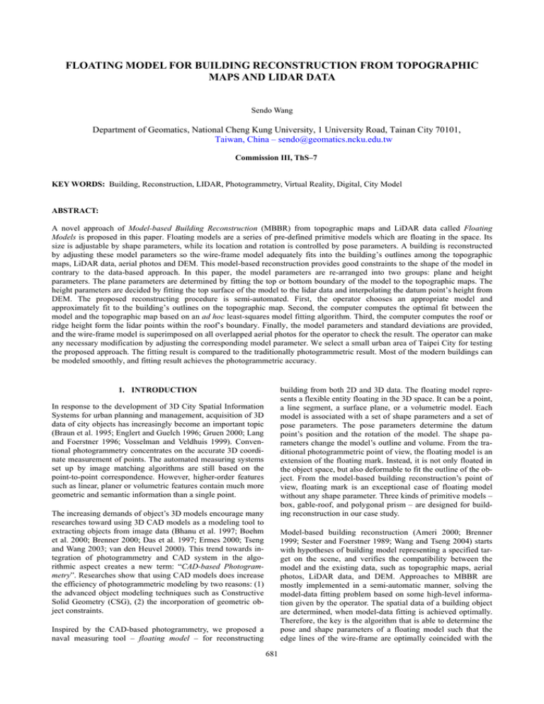
FLOATING MODEL FOR BUILDING RECONSTRUCTION FROM TOPOGRAPHIC
MAPS AND LIDAR DATA
Sendo Wang
Department of Geomatics, National Cheng Kung University, 1 University Road, Tainan City 70101,
Taiwan, China – sendo@geomatics.ncku.edu.tw
Commission III, ThS–7
KEY WORDS: Building, Reconstruction, LIDAR, Photogrammetry, Virtual Reality, Digital, City Model
ABSTRACT:
A novel approach of Model-based Building Reconstruction (MBBR) from topographic maps and LiDAR data called Floating
Models is proposed in this paper. Floating models are a series of pre-defined primitive models which are floating in the space. Its
size is adjustable by shape parameters, while its location and rotation is controlled by pose parameters. A building is reconstructed
by adjusting these model parameters so the wire-frame model adequately fits into the building’s outlines among the topographic
maps, LiDAR data, aerial photos and DEM. This model-based reconstruction provides good constraints to the shape of the model in
contrary to the data-based approach. In this paper, the model parameters are re-arranged into two groups: plane and height
parameters. The plane parameters are determined by fitting the top or bottom boundary of the model to the topographic maps. The
height parameters are decided by fitting the top surface of the model to the lidar data and interpolating the datum point’s height from
DEM. The proposed reconstructing procedure is semi-automated. First, the operator chooses an appropriate model and
approximately fit to the building’s outlines on the topographic map. Second, the computer computes the optimal fit between the
model and the topographic map based on an ad hoc least-squares model fitting algorithm. Third, the computer computes the roof or
ridge height form the lidar points within the roof’s boundary. Finally, the model parameters and standard deviations are provided,
and the wire-frame model is superimposed on all overlapped aerial photos for the operator to check the result. The operator can make
any necessary modification by adjusting the corresponding model parameter. We select a small urban area of Taipei City for testing
the proposed approach. The fitting result is compared to the traditionally photogrammetric result. Most of the modern buildings can
be modeled smoothly, and fitting result achieves the photogrammetric accuracy.
building from both 2D and 3D data. The floating model represents a flexible entity floating in the 3D space. It can be a point,
a line segment, a surface plane, or a volumetric model. Each
model is associated with a set of shape parameters and a set of
pose parameters. The pose parameters determine the datum
point’s position and the rotation of the model. The shape parameters change the model’s outline and volume. From the traditional photogrammetric point of view, the floating model is an
extension of the floating mark. Instead, it is not only floated in
the object space, but also deformable to fit the outline of the object. From the model-based building reconstruction’s point of
view, floating mark is an exceptional case of floating model
without any shape parameter. Three kinds of primitive models –
box, gable-roof, and polygonal prism – are designed for building reconstruction in our case study.
1. INTRODUCTION
In response to the development of 3D City Spatial Information
Systems for urban planning and management, acquisition of 3D
data of city objects has increasingly become an important topic
(Braun et al. 1995; Englert and Guelch 1996; Gruen 2000; Lang
and Foerstner 1996; Vosselman and Veldhuis 1999). Conventional photogrammetry concentrates on the accurate 3D coordinate measurement of points. The automated measuring systems
set up by image matching algorithms are still based on the
point-to-point correspondence. However, higher-order features
such as linear, planer or volumetric features contain much more
geometric and semantic information than a single point.
The increasing demands of object’s 3D models encourage many
researches toward using 3D CAD models as a modeling tool to
extracting objects from image data (Bhanu et al. 1997; Boehm
et al. 2000; Brenner 2000; Das et al. 1997; Ermes 2000; Tseng
and Wang 2003; van den Heuvel 2000). This trend towards integration of photogrammetry and CAD system in the algorithmic aspect creates a new term: “CAD-based Photogrammetry”. Researches show that using CAD models does increase
the efficiency of photogrammetric modeling by two reasons: (1)
the advanced object modeling techniques such as Constructive
Solid Geometry (CSG), (2) the incorporation of geometric object constraints.
Model-based building reconstruction (Ameri 2000; Brenner
1999; Sester and Foerstner 1989; Wang and Tseng 2004) starts
with hypotheses of building model representing a specified target on the scene, and verifies the compatibility between the
model and the existing data, such as topographic maps, aerial
photos, LiDAR data, and DEM. Approaches to MBBR are
mostly implemented in a semi-automatic manner, solving the
model-data fitting problem based on some high-level information given by the operator. The spatial data of a building object
are determined, when model-data fitting is achieved optimally.
Therefore, the key is the algorithm that is able to determine the
pose and shape parameters of a floating model such that the
edge lines of the wire-frame are optimally coincided with the
Inspired by the CAD-based photogrammetry, we proposed a
naval measuring tool – floating model – for reconstructing
681
The International Archives of the Photogrammetry, Remote Sensing and Spatial Information Sciences. Vol. XXXVII. Part B3b. Beijing 2008
ordinate system defines the model space and X-Y-Z coordinate
system defines the object space. The little pink sphere indicates
the datum point of the model. The yellow primitive model is in
the original position and pose, while the grey model depicts the
position and pose after changing pose parameters (dX, dY, dZ, t,
s, α). It is very clear that, the model is “floating” in the space by
controlling these pose parameters. The volume and shape of the
model remain the same while the pose parameters change. The
shape parameters describe the shape and size of the primitive
model, e.g., a box has three shape parameters: width (w), length
(l), and height (h). Changing the values of shape parameters
elongates the primitive in the three dimensions, but still keeps
its shape as a rectangular box. Various primitive may be associated with different shape parameters, e.g., a gable-roof house
primitive has an additional shape parameter – roof’s height (rh).
Fig. 3 shows three examples from each type of models with the
change of shape parameters. The point is an exceptional case
that does not have any shape parameters. Fig. 3 points out the
other important characteristic of the floating model – the flexible shape with certain constraints. Changing the shape parameters does not affect the position or the pose of the model.
corresponding edge pixels. To deal with this problem, we proposed a tailored Least-squares Model-data Fitting (LSMDF)
algorithm as a major component of the building reconstruction
framework.
To simplify the fitting problem, the model parameters are rearranged into two groups, plane and height parameters. Hence the
model-data fitting procedures are also divided into three steps.
First, fit model to topographic maps to derive plane parameters.
Second, interpolate datum’s height from DEM and fit model to
LiDAR data to derive height parameters. Finally, the wireframe
model is projected onto aerial photos for examining. The operator can make further modification of the model according to the
photos if necessary. Fig. 1 uses a box model as an example to
depict the proposed reconstruction procedures. The hexagons
depict the information required from the data sources. The parameters labeled in red color are the varied ones during the procedure.
Topographic Maps
Building
Boundary
LiDAR Data &
DEM
Aerial
Photos
Ground &
Roof Height
Building
Images
Z'
Z
α
Y
Plane Fitting
l=1
w=1
h=1
dX=0
dY=0
dZ=0
α=0
Height Fitting
l=19.1
w=4.4
h=1.0
dX=304660.5
dY=2761940.2
dZ=0.0
α=121.7
t
dY
Z'
Y
w
Figure 1. The flowchart of the reconstructing procedures.
Rect angle
l
2. FLOATING MODELS
dX
t
dZ
X'
X
Line Segment
Z'
Z
w'
s
h
dY
Bo x
l'
h'
Y'
t
dY
X'
w'
s
dZ
dX
l
X
Rectangle Plane
s
Bo x
α
Y
w
X'
t
l'
dY
l
ng le
Recta
Y'
dZ
dX
Y' l'
α
α
Y
X
Point
Z
Z'
Z
X'
s
dZ
dX
Final Examining
l=19.1
l=19.1
w=4.4
w=4.4
h=22.7
h=22.7
dX=304660.5
dX=304660.5
dY=2761940.2
dY=2761940.
dZ=23.9
2
α=121.7
dZ=23.9
α 121 7
Y'
X
Box
Figure 2. Adjusting the pose parameters of floating models.
Traditional photogrammetric mapping systems concentrate on
the accurate measurement of points. The floating mark is a simple way to represent the position of a point in the space, and
thus, has been served as the only measuring tool on the stereo
plotters up to nowadays. However, the floating mark reaches its
limits when the conjugate points can not be identified due to the
occlusions or interferences from other noises. And with the increasing needs of 3D object models, point-by-point measurement has been become the bottleneck of the production. To deal
with the modeling problem, we proposed floating models which
complies with the constructive solid geometry. The floating
model is basically a primitive CSG model, which determines
the intrinsic geometric property of a part of building. That can
be categorized into four types: point, linear feature, plane, or
volumetric solid. Each type contains various primitive models
for the practical needs. For example, the linear feature includes
the line segment. The plane includes the rectangle, the circle,
the triangle, etc. The volumetric solid includes the box, the gable-roof house, etc. Despite the variety in their shape, each
primitive model commonly has a datum point, and is associated
with a set of pose parameters and a set of shape parameters. The
datum point and the pose parameter determine the position of
the floating model in object space. It is adequate to use 3 translation parameters (dX, dY, dZ) to represent the position and 3
rotation parameters, tilt (t) around Y-axis, swing (s) around Xaxis, and azimuth (α) around Z-axis to represent the rotation of
a primitive model. Fig. 2 shows four examples from each type
of models with the change of the pose parameters. X’-Y’-Z’ co-
l'
l'
h'
l'
w'
l
Line Segment
l
Rectangle Plane
h
w'
l
Box Solid
Figure 3. Adjusting the shape parameters of floating models.
3. LEAST-SQUARES MODEL-DATA FITTING
Since the topographic maps are plotted by photogrammetric
techniques, its plane accuracy would be better than the LiDAR
data. On the contrary, the LiDAR data provides better height
accuracy. Therefore, the proposed model-data fitting procedures
are separated into two steps: (1) the plane parameters are derived by fitting model’s bottom to the topographic map; (2) the
height parameters are derived by fitting model’s roof to the LiDAR data.
The objective of the plane fitting is the building’s boundary on
the topographic map. However, the map contains much more
elements than building boundaries. A “clean & build” process is
necessary to establish the close-and-complete polygons of only
buildings. These polygons are the bases of plane fitting. The
operator selects an appropriate primitive model and makes the
approximately fit according to the polygon to be measured. The
corresponding polygon’s boundary is then re-sampled as sample
682
The International Archives of the Photogrammetry, Remote Sensing and Spatial Information Sciences. Vol. XXXVII. Part B3b. Beijing 2008
the distance dij represents a discrepancy between a sample point
Tij and its corresponding edge vmvn, which is expected to be
zero. Therefore, the objective of the fitting function is to minimize the squares sum of dij. Suppose an edge is composed of
the vertices vm(xm, yn) and vn(xn, yn), and there is an edge pixel
Tij(xij, yij) located inside the buffer. The distance dij from the
point Tij to the edge vmvn can be formulated as the following
equation:
( y m − y n ) xij + ( xn − xm ) yij + ( y n xm − y m xn )
d ij =
( xm − xn ) 2 + ( y m − y n ) 2
(1)
points with fixed interval. Each sample point would be treated
as an observation in the LSMDF to solve the plane parameters
as optimal fit. Fig. 4 depicts the flowchart of the plane fitting.
Data
Process
Example
3R
Topographic
Maps
Pre-Process
5R
Building
Boundary
The coordinates of vertices vm(xm, ym) and vn(xn, yn) are functions of the unknown plan parameters. Therefore, dij will be a
function of the plan parameters. Taking a box model for instance, dij will be a function of w, l, α, dX, and dY, with the hypothesis that a normal building rarely has a tilt angle (t) or
swing angle (s). The least-squares solution for the unknown parameters can be expressed as:
Manual Fitting
Approximate
Plane Parameters
Resample
Σdij2 = Σ[Fij ( w, l, α, dX, dY)]2 → min.
Eq.(2) is a nonlinear function with regard to the unknowns, so
that the Newton’s method is applied to solve for the unknowns.
The nonlinear function is differentiated with respect to the unknowns and becomes a linear function with regard to the increments of the unknowns as follows:
Sample Points
Optimal Fitting
Optimal Plane
Parameters
0 + v ij = Fij 0 + (
(
Figure 4. The flowchart of plane fitting.
Since the model has been manually fit, the bottom edges of the
wireframe model should be close to the building’s boundary on
the map. Benefited from the approximate fitting, the LSMDF
iteratively pulls the model to the optimal fit instead of blindly
searching for the solution. To avoid the disturbance of irrelevant
sample points, only those points distributed within a specified
buffer zone are adopted for fitting calculation. Figure 5 depicts
the sample point Tij and a wbuffer wide buffer determined by an
edge vmvn of the model. The suffix i is the index of edge line Li
and j is the index of sample points. Filtering edge pixels with
buffer is reasonable, because the discrepancies between the bottom edges and the corresponding sample points should be small,
as the model parameters have been fit approximately. However,
the buffer size has to be carefully chosen because it will directly affect the convergence of the computation.
Discard Sample Points
y
Adopted Sample Points
v n( x n, y n)
T ij( x ij , y ij)
Ed
Bu
ge
ffe
L
ff e
el
r
d ij
bu
od
i
r
r
v m ( x m, y m)
x
wb
uf
fe
∂Fij
∂dY
∂Fij
∂l
) 0 ∆l + (
) 0 ∆dY + (
∂Fij
∂dZ
∂Fij
∂w
) 0 ∆w + (
) 0 ∆dZ + (
∂Fij
∂dX
∂Fij
∂α
) 0 ∆dX +
) 0 ∆α
(3)
in which, Fij0 is the approximation of the function Fij calculated
with given approximations of the unknown parameters. Given a
set of unknown approximations, the least-squares solution for
the unknown increments can be solved, and the approximations
are updated by the increments. Repeating this calculation, the
unknown parameters can be solved iteratively.
The linearized equations can be expressed as a matrix form:
V=AX-L, where A is the matrix of partial derivatives; X is the
vector of the increments; L is the vector of approximations; and
V is the vector of residuals. The objective function actually can
be expressed as q=VTV →min. For each iteration, X can be
solved by the matrix operation: X=(ATA)-1ATL. The standard
deviation of each increment can also be calculated as the accuracy index of the LSMDF.
The objective of the height fitting is the building’s roof in the
LiDAR data. As the distance from sample point to the edge is
the observation function in the plane fitting, the observation
function should be the distance from LiDAR point to the roof
plane in the height fitting. The roof plane equation is composed
of model parameters. However, the calculations of 3D fitting
would be much more complicated than 2D. And it will also increase the iteration number and the chance to divergence. Considering the efficiency and the practicality, we adopt an easier
method for the height fitting in this paper. Since the plane parameters have been fit optimally, LiDAR points within the
plane range are supposed to belong to the model. These points
are then projected to a local 2D coordinate system which is defined on the façade of the model. Fig. 6 illustrates the transformation of a ridge-roof building. Thus the observation function
is simplified as the distance from 2D point to edge, similar to
the plan fitting.
w
M
(2)
Figure 5. Buffer zone for fitting.
The fitting condition we are looking for is that the model edge
exactly falls on the building boundary on the map. In Eq.(1),
683
The International Archives of the Photogrammetry, Remote Sensing and Spatial Information Sciences. Vol. XXXVII. Part B3b. Beijing 2008
building reconstructed by box and polyhedral prism models.
For the whole test area, two operators worked for one week and
totally reconstructed 4130 buildings. Fig. 9 shows a part of the
reconstructed city model. We select 30 buildings for correctness
and accuracy evaluation. These models are first evaluated in
their shape with aerial and terrestrial photos by human eyes.
The correctness rate is about 88.5%. Then, the vertices coordinates of the 30 building models are calculated from model parameters and then compared to the photogrammetric and ground
survey result. Table 1 lists the statistics of the coordinate differences. The larger X-Y differences most due to the mismatch
point, while the larger Z differences most due to the parapets.
Figure 6. Projection of the LiDAR points for height Fitting.
4. EXPERIMENTS
A small urban area of Taipei City about 500hectare is selected
for testing. The 1/1000 scale digital topographic maps have
been pre-proceeded to generate building polygons. The grid interval of the corresponding DEM is 4m. The point density of
LiDAR point cloud is about 10 points within 1m2, which is
good enough to reconstruct normal building roofs. The aerial
photos are taken by the Vexcel UltraCam D photogrammetric
camera. The focal length is 101.4mm, the image size is
7500*11500pixel, and the size of a pixel is 9*9µm. The average
flight height is about 1930m, so the ground resolution is about
0.17m/pixel. Meanwhile, we develop a PC program by C++
language to implement the proposed building reconstruction
procedures. The interface is illustrated by Fig. 7. The operating
sequences are as follow: (1) observe the topographic map in the
left window and select the appropriate model; (2) click vertices
v1, v2, and v3 in sequences on the topographic map to give initial
parameters; (3) examine projections on photos and adjust the
model parameters if needed; (4) click the Fitting button to implement LSMDF of plane and height optimal fitting; (5) examine projections on photos and adjust the model parameters if
needed; (6) output and save the model parameters. A model is
usually reconstructed within a minute, but the time for a building depends on its complexity.
Table 1. Statistics of coordinates differences.
Coordinates Differences
Average(m)
Avg. of Absolute Values(m)
Std. Deviation (m)
∆X
0.051
0.236
0.2953
∆Y
0.110
0.294
0.3490
∆Z
-0.0146
0.8816
1.1400
Figure 9. A part of the reconstructed 3D building models.
Resulting from our experiments, most of the modern buildings
can be modeled smoothly, and fitting result achieves the photogrammetric accuracy. However, some of the buildings are illegally reconstructed into an arbitrarily shape, which makes it difficult to be modeled by our pre-defined model. In that case, the
building should be decomposed into several parts for fitting and
then aggregate into one composite model. For some traditional
Chinese architecture, it is very difficult to reconstruct their
curvy eaves by our pre-defined model. Fig. 10 shows an example, in which the building can only be reconstructed approximately.
Figure 7. The program interface of MBBR.
Figure 10. Curvy eaves can only be reconstructed approximately.
Figure 8. A complex building model reconstructed by box and
polyhedral prism models.
Our system currently provides three kinds of model for reconstructing most of the modern buildings: box, gable-roof, and
polyhedral prism model. A building model is composed of several primitive models. Fig. 8 shows an example of a complex
5. CONCLUSIONS
The floating model is proposed as a model-based building reconstruction approach, which is a flexible 3D measuring tool
684
The International Archives of the Photogrammetry, Remote Sensing and Spatial Information Sciences. Vol. XXXVII. Part B3b. Beijing 2008
Brenner, C., 2000. Towards Fully Automatic Generation of
City Models. In: The International Archives of the
Photogrammetry, Remote Sensing and Spatial Information
Sciences, Amsterdam, the Netherlands, Vol. XXXIII, Part B3,
pp. 85-92.
floating in the object space. This paper introduces one kind of
its utilization for reconstructing models from different source
data. Plan parameters are fit from topographic maps and height
parameters are fit from LiDAR data and DEM. Aerial Photos
are also used for examining and modifying. According to our
case study of Taipei City, the procedure goes smoother and
faster with the increase of operating experiences. Here are some
characteristics of the proposed approach:
Das, S., Bhanu, B. and Ho, C.-C., 1997. Generic Object
Recognition Using CAD-Based Multiple Representations. in:
IEEE CAD-Based Vision Workshop, pp. 202-209.
1. For most of the normal buildings, floating model does
increase efficiency than point-by-point measurement.
2. The labour-consuming precise measurement is carried out
by computer while the operator only needs to select
model and approximately fit it.
3. The inner constraints guarantees the geometric nature
unchanged after reconstructing.
4. It is possible to reconstruct the whole building even if a
part of it is occluded.
Englert, R. and Gülch, E., 1996. One-eye Stereo System for the
Acquisition of Complex 3D Building Descriptions. GIS, No. 4,
pp. 1-11.
Ermes, P., 2000. Constraints in CAD Models for Reverse
Engineering Using Photogrammetry. In: The International
Archives of the Photogrammetry, Remote Sensing and Spatial
Information Sciences, Amsterdam, the Netherlands, Vol.
XXXIII, Part B5/1, pp. 215-221.
However, we also find some shortcomings of the model-based
approach:
Grün, A., 2000. Semi-automated Approaches to Site Recording
and Modeling. In: The International Archives of the
Photogrammetry, Remote Sensing and Spatial Information
Sciences, Amsterdam, the Netherlands, Vol. XXXIII, Part B5,
pp. 309-318.
1. A building could never be reconstructed correctly if there
is no adequate primitive model.
2. The decomposition of building needs practice and
experience.
3. It is difficult to implement the subtraction operation
between two models.
4. For those very complicated buildings, model-based
approach will cost more time than data-based approach.
Lang, F. and Förstner, W., 1996. 3D-City Modeling with a
Digital One-eye Stereo System, In: The International Archives
of the Photogrammetry, Remote Sensing and Spatial
Information Sciences, Vienna, Austria, Vol. XXXI, pp. 415-420.
Sester, M. and Förstner, W., 1989. Object Location Based on
Uncertain Models, Mustererkennung 1989. Informatik
Fachberichte 219. Springer Verlag, pp. 457-464.
Therefore, we suggest two further research objectives: (1) designing more primitive models such as curvy plane. (2) analyzing the topology and implement the Boolean operator among
3D models.
Tseng, Y.-H. and Wang, S., 2003. Semiautomated Building
Extraction
Based
on
CSG
Model-Image
Fitting.
Photogrammetric Engineering & Remote Sensing, 69(2), pp.
171-180.
REFERENCES
van den Heuvel, F. A., 2000. Trends in CAD-based
Photogrammetric Measurement. In: The International Archives
of the Photogrammetry, Remote Sensing and Spatial
Information Sciences, Amsterdam, the Netherlands, Vol.
XXXIII, Part B5, pp. 852-863.
Ameri, B., 2000. Feature Based Model Verification (FBMV): A
New Concept for Hypothesis Validation in Building
Reconstruction. In: The International Archives of the
Photogrammetry, Remote Sensing and Spatial Information
Sciences, Amsterdam, the Netherlands, Vol. XXXIII, Part B3/1,
pp. 24-35.
Bhanu, B., Dudgeon, D. E., Zelnio, E. G., Rosenfeld, A.,
Casasent, D., and Reed, I. S., 1997. Guest Editorial
Introduction to the Special Issue on Automatic Target Detection
and Recognition. IEEE Transactions on Image Processing, 6(1),
pp. 1-6.
Böhm, J., Brenner, C., Gühring, J. and Fritsch, D., 2000.
Automated Extraction of Features from CAD Models for 3D
Object Recognition. In: The International Archives of the
Photogrammetry, Remote Sensing and Spatial Information
Sciences, Amsterdam, the Netherlands, Vol. XXXIII, Part B5,
pp. 76-83.
Braun, C., Kolbe, T. H., Lang, F., Schickler, W., Steinhage, V.,
Cremers, A. B., Förstner, W., and Plümer, L., 1995. Models for
Photogrammetric Building Reconstruction. Computers &
Graphics, 19(1), pp. 109-118.
Brenner, C., 1999. Interactive Modelling Tools for 3D Building
Reconstruction. In: Photogrammetric Week '99. Wichmann,
Stuttgart, pp. 23-34.
685
Vosselman, G. and Veldhuis, H., 1999. Mapping by Dragging
and Fitting of Wire-Frame Models. Photogrammetric
Engineering & Remote Sensing, 65(7), pp. 769-776.
Wang, S. and Tseng, Y.-H., 2004. Least-squares Model-image
Fitting for Building Extraction from Aerial Images. Asian Journal of Geoinformatics, 4(4), pp. 3-12.
The International Archives of the Photogrammetry, Remote Sensing and Spatial Information Sciences. Vol. XXXVII. Part B3b. Beijing 2008
686