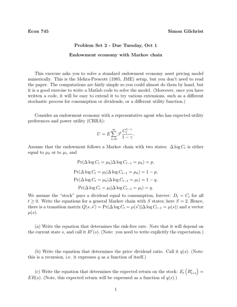
Econ 745
Simon Gilchrist
Problem Set 2 - Due Tuesday, Oct 1
Endowment economy with Markov chain
This exercise asks you to solve a standard endowment economy asset pricing model
numerically. This is the Mehra-Prescott (1985, JME) setup, but you don’t need to read
the paper. The computations are fairly simple so you could almost do them by hand, but
it is a good exercise to write a Matlab code to solve the model. (Moreover, once you have
written a code, it will be easy to extend it to try various extensions, such as a different
stochastic process for consumption or dividends, or a different utility function.)
Consider an endowment economy with a representative agent who has expected utility
preferences and power utility (CRRA):
U =E
∞
X
t=0
βt
Ct1−γ
.
1−γ
Assume that the endowment follows a Markov chain with two states: ∆ log Ct is either
equal to µh or to µl , and
Pr(∆ log Ct = µh |∆ log Ct−1 = µh ) = p,
Pr(∆ log Ct = µl |∆ log Ct−1 = µh ) = 1 − p,
Pr(∆ log Ct = µh |∆ log Ct−1 = µl ) = 1 − q,
Pr(∆ log Ct = µl |∆ log Ct−1 = µl ) = q.
We assume the “stock” pays a dividend equal to consumption, forever: Dt = Ct for all
t ≥ 0. Write the equations for a general Markov chain with S states; here S = 2. Hence,
there is a transition matrix Q(s, s0 ) = Pr(∆ log Ct = µ(s0 )|∆ log Ct−1 = µ(s)) and a vector
µ(s).
(a) Write the equation that determines the risk-free rate. Note that it will depend on
the current state s, and call it Rf (s). (Note: you need to write explicitly the expectation.)
(b) Write the equation that determines the price–dividend ratio. Call it q(s). (Note:
this is a recursion, i.e. it expresses q as a function of itself.)
e
(c) Write the equation that determines the expected return on the stock: Et Rt+1
=
ER(s). (Note, this expected return will be expressed as a function of q(s).)
1
(d) Consider the following parameters:
S = 2, µh = 1.02, µl = .98,
p = q = .95, β = .98, γ = 2.
Compute the risk-free rate, the price-dividend ratio, and the expected return and
the expected excess return conditional on each state. (Note, you will need to compute
explicitly the expectations of questions (a)-(b)-(c), and solve the recursion of q(s) just
like you solve a Bellman equation.)
(e) Compute the unconditional expected return and excess return on the stock. To do
so, you need to use the invariant (or ergodic) distribution, which gives you the probability
that each state is reached. The invariant distributon υ(s) satisfies the linear system:
∀s0 = 1...S : υ(s0 ) =
S
X
Q(s, s0 )υ(s).
s=1
If you want more details on Markov chains, see my notes http://people.bu.edu/fgourio/markov.pdf
(f) Produce a plot, as a function of γ, of the unconditional excess return on the
stock. Also produce a plot of the unconditional volatility of the stock return, and the
unconditional risk-free rate.
(g) Calibration: for a two-state Markov chain with transition
p
1−p
1−q
q
!
,
and means (µh , µl ), with µh = µ + δ and µl = µ − δ, compute the mean, variance,
and serial correlation of the process. We can measure these statistics in U.S. data for
consumption growth, and then find p, q, δ, to replicate these statistics, so that our implied
time series process for ∆ log Ct is similar to the data. In U.S. data, typical numbers
would be for annual consumption growth: E(∆ log Ct ) = 2%, var(∆ log Ct ) = 0.0006,
and ρ(∆ log Ct ) = −.1. What are the implied δ, p, q?
2