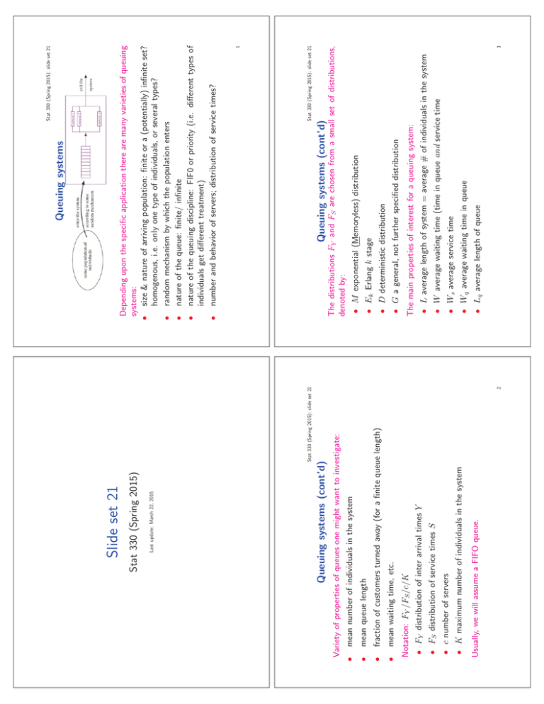
mean queue length
fraction of customers turned away (for a finite queue length)
mean waiting time, etc.
•
•
•
Usually, we will assume a FIFO queue.
• K maximum number of individuals in the system
• c number of servers
• FS distribution of service times S
• FY distribution of inter arrival times Y
Notation: FY /FS /c/K
mean number of individuals in the system
•
Variety of properties of queues one might want to investigate:
2
Stat 330 (Spring 2015): slide set 21
Queuing systems (cont’d)
Last update: March 22, 2015
Stat 330 (Spring 2015)
Slide set 21
Stat 330 (Spring 2015): slide set 21
• Lq average length of queue
• Wq average waiting time in queue
• Ws average service time
• W average waiting time (time in queue and service time
• L average length of system = average # of individuals in the system
The main properties of interest for a queuing system:
• G a general, not further specified distribution
• D deterministic distribution
• Ek Erlang k stage
• M exponential (Memoryless) distribution
Queuing systems (cont’d)
3
The distributions FY and FS are chosen from a small set of distributions,
denoted by:
Stat 330 (Spring 2015): slide set 21
1
Depending upon the specific application there are many varieties of queuing
systems:
• size & nature of arriving population: finite or a (potentially) infinite set?
homogenous, i.e. only one type of individuals, or several types?
• random mechanism by which the population enters
• nature of the queue: finite/ infinite
• nature of the queuing discipline: FIF0 or priority (i.e. different types of
individuals get different treatment)
• number and behavior of servers; distribution of service times?
Queuing systems
Stat 330 (Spring 2015): slide set 21
Relationship between properties
where
6
For c servers and an overall capacity of K (where K may be = ∞) the
transition diagram looks like this:
A way to visualize what is going on in the queuing system is the birth &
death transition diagram.
pk = limt→∞ P (N (t) = k).
7
The problem of finding the steady state probabilities of the B&D process
is equivalent to finding the steady state probabilities for the number of
individuals in the queuing system,
This ratio is called the traffic intensity a. For a M/M/1 queuing system,
the traffic intensity is constant for all k.
Let N (t) denote the number of individuals in the system at time t, N (t)
can then be modeled using a Birth & Death process:
λk = birth rate = arrival rate = λ for all k
μk = death rate = service rate = μ for all k
We’ve already seen that the ratio λ/μ is very important for the analysis of
the B&D process.
Situation: exponential inter arrival times with rate λ, exponential service
times with rate μ.
Stat 330 (Spring 2015): slide set 21
Stat 330 (Spring 2015): slide set 21
Birth & Death Transition Diagrams
5
The M/M/1 Queue
To choose the easier way of computation, the following overview of the
relationships between these properties helps:
4
λ̄ is the average rate at which individuals enter the system.
W is the average time spent in the system, and
L is the average number of individuals in the system,
L = λ̄ · W
Little’s Law: For a queuing system in steady state
For computing the properties L, W, Ws, Wq , Lq there are usually two
different ways: an easy way and a difficult one.
Ls = λ¯s · Ws.
• This gives us a way to analyze the queuing systems using the methods
from the previous chapter.
This theorem can also be applied to the queue itself:
Lq = λ¯q · Wq
or to the server
• The theorem below links waiting times to the number of people in the
system and will be very useful in the future
Stat 330 (Spring 2015): slide set 21
More on Little’s Theorem
• We model the number of individuals in the system at time t as the Birth
& Death Process X(t)
• The main idea of a queuing system is to model the number of individuals
in the system (queue and server) as a Birth & Death Process.
Model queueing systems as Stochastic processes
Stat 330 (Spring 2015): slide set 21
= ak (1 − a)
Wq = W − Ws =
1
·
μ
1
−1
1−a
=
1 a
.
μ1 − a
10
Since we know that service times are exponentially distributed with rate μ,
the the average waiting time is Ws = μ1 .
Thus, the closer the service rate is to the arrival rate, the larger is the
expected number of people in the system.
a2
1−a
11
Clearly, the distribution of the waiting times depends on the number of
individuals already in the queue at time t.
Distribution of time in the queue: Denote by q(t) the time that an individual
entering the system at time t has to spend waiting in the queue.
This is the server utilization rate.
Further we see, that the long run probability that the server is busy is given
as:
P (server busy) = 1 − P (system empty) = 1 − p0 = a.
L q = Wq λ =
The average length of the queue is, using Little’s Law again, is:
The M/M/1 Queue (cont’d)
Stat 330 (Spring 2015): slide set 21
The overall time spent in the system is a sum of the time spent in the
queue Wq and the average time spent in service Ws i.e. W = Wq + Ws
Thus, the average time spent waiting in the queue is:
1
a
.
−1=
1−a
1−a
Stat 330 (Spring 2015): slide set 21
The mean time spent in the queueing system, W is then, using Little’s Law:
1
1
·
μ 1−a
t→∞
Note that L gets larger as a gets closer to 1, that is, as the service rate
gets closer to the arrival rate.
t→∞
L = lim E[N (t)] = lim E[N (t) + 1] − 1 =
The average number of individuals in the queuing system, L, is
limt→∞ E[N (t)]:
We can use that to get the expected value of N (t):
It is a modified geometric distribution, as N (t) can be 0 (empty system).
Thus N (t) + 1 has a Geometric distribution Geo(1 − a).
9
The M/M/1 Queue (cont’d)
W = L/λ =
Stat 330 (Spring 2015): slide set 21
The M/M/1 Queue (cont’d)
8
N (t) therefore has a (modified) geometric distribution for large t!
pk
...
p3 = a3(1 − a)
p2 = a2(1 − a)
p1 = a(1 − a)
p0 = 1 − a
We have a system with a steady state if a < 1.
∞
1
If a < 1 S = k=0 ak = 1−a
, then
The B&D balance equations then say that 1 = p0(1 + a + a2 + . . .)
The M/M/1 Queue (cont’d)
Stat 330 (Spring 2015): slide set 21
for large t
12
We can put those pieces together in order to get the large t distribution for
q(t) using the the total probability law.
q(t)|X(t) = k ∼ Erlang(k, μ)
This is a conditional distribution, since it is the distribution of q(t) given
that the number of people in the system is k:
If there are k individuals in the queue, the waiting time q(t) is Erlang(k, μ)
(i.e., k departures with departures occurring with a rate of μ).
limt→∞ P (q(t) = 0) = p0 = 1 − a.
For large t we therefore get:
The individual entering the system doesn’t have to wait at all in the queue
when the system at time t is empty.
The M/M/1 Queue (cont’d)
=
−x/W
1 − ae
,
=
k=1
∞
k−1
j
−μx (xμ)
p0 +
(1 −
e
)pk = . . .
j!
j=0
k=1
∞
(1 − P oμx(k − 1))pk
P (q(t) ≤ x|X(t) = k)pk
P (q(t) ≤ x ∩ X(t) = k)
1
μ
1
· 1−a
=
now use total probability law!
p0 +
k=0
∞
k=0
∞
P (q(t) ≤ x) =
=
=
=
=
where W is the average time spent in the system, W =
Fq(t)(x)
For large t and x ≥ 0:
1
μ−λ .
13
Stat 330 (Spring 2015): slide set 21
The M/M/1 Queue (cont’d)