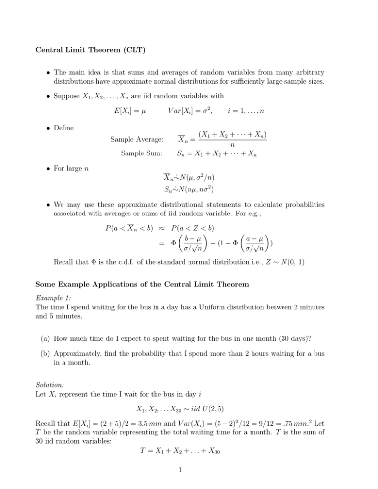
Central Limit Theorem (CLT)
• The main idea is that sums and averages of random variables from many arbitrary
distributions have approximate normal distributions for sufficiently large sample sizes.
• Suppose X1 , X2 , . . . , Xn are iid random variables with
E[Xi ] = µ
• Define
Sample Average:
Sample Sum:
V ar[Xi ] = σ 2 ,
i = 1, . . . , n
(X1 + X2 + · · · + Xn )
n
Sn = X1 + X2 + · · · + Xn
Xn =
• For large n
X n ∼N
˙ (µ, σ 2 /n)
Sn ∼N
˙ (nµ, nσ 2 )
• We may use these approximate distributional statements to calculate probabilities
associated with averages or sums of iid random variable. For e.g.,
P (a < X n < b) ≈ P (a < Z < b)
b−µ
a−µ
√
√ )
= Φ
− (1 − Φ
σ/ n
σ/ n
Recall that Φ is the c.d.f. of the standard normal distribution i.e., Z ∼ N (0, 1)
Some Example Applications of the Central Limit Theorem
Example 1:
The time I spend waiting for the bus in a day has a Uniform distribution between 2 minutes
and 5 minutes.
(a) How much time do I expect to spent waiting for the bus in one month (30 days)?
(b) Approximately, find the probability that I spend more than 2 hours waiting for a bus
in a month.
Solution:
Let Xi represent the time I wait for the bus in day i
X1 , X2 , . . . X30 ∼ iid U (2, 5)
Recall that E[Xi ] = (2 + 5)/2 = 3.5 min and V ar(Xi ) = (5 − 2)2 /12 = 9/12 = .75 min.2 Let
T be the random variable representing the total waiting time for a month. T is the sum of
30 iid random variables:
T = X1 + X2 + . . . + X30
1
(a) We need E[T ]. The CLT tells us that E[T ] = nµ where µ = E[Xi ]. Thus E[T ] =
30 × 3.5 = 105 min. We may also compute this from scratch as follows:
E[T ] = E[X1 + X2 + . . . + X30 ]
= E[X1 ] + E[X2 ] + . . . + E[X30 ]
= µ + µ + . . . + µ = 30 × 3.5 = 105 min.
(b) From the CLT, we have
T ∼N
˙ (30 × 3.5, 30 × 0.75) i.e. T ∼N
˙ (105, 22.5)
We need the probability that T is greater than 120 minutes, i.e., P (T > 120)
P (T > 120) = 1 − P (T ≤ 120)
(120 − 105)
√
≈ 1 − P (Z ≤
) by CLT
22.5
= 1 − Φ(3.16) = 1 − .9992112 = .00079
Example 2:
An astronmer wants to measure the distance, d, from the observatory to a star. Due to the
variation of atmospheric conditions and imperfections in the measurement method, a single
measurement will not produce the exact distance d. The astronomer takes n measurements of
the distance and uses the sample average to estimate the true distance. From past records of
these measurements the astronomer knows the variance of a single measurement is 4parsec2 .
How many measurement should the astronomer make so that the chance that his estimate
differs by d by more than .5 parsecs is at most .05?
Solution:
Let Xi be the ith measurement. The astronomer assumes that
X1 , X2 , . . . Xn ∼ iid with E[Xi ] = d and V ar[Xi ] = 4
The estimate of d is
(X1 + X2 + · · · + Xn )
n
We want to find the number of measurements n so that
Xn =
P (|X n − d| > .5) ≤ .05
We know that
P (|X n − d| > .5) = P (X n − d > .5) + P (X n − d < −.5)
We use the CLT to approximate each of the probabilities on the right. From the CLT we
have that
X n ∼N
˙ (d, 4/n)
2
Thus
P (|X n − d| > .5) = P (X n − d > .5) + P (X n − d < −.5)
!
!
Xn − d
.5
Xn − d
−.5
>p
<p
= P p
+P p
4/n
4/n
4/n
4/n
!
!
−.5
.5
+P Z < p
≈ P Z>p
4/n
4/n
√
√
= 1 − Φ( n/4) + Φ(− n/4)
√
= 2(1 − Φ( n/4))
√
We need to find √
an integer n so that 2(1 − Φ( n/4)) is just less than or equal to .05. We
n∗ and take the required number
of measurements
will set 2(1 − Φ( n∗ /4)) = .05, solve for
√
√
∗
to be the dn e. Observe that 2(1√− Φ( n/4)) = .05 implies that Φ( n/4)) = .975. Using
the Normal cdf tables, this gives n/4 = 1.96; thus n∗ = 61.47. Thus the astronomer must
take at least 62 measurements to have the accuracy specified above.
3