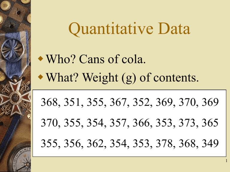
Quantitative Data
Who? Cans of cola.
What? Weight (g) of contents.
368, 351, 355, 367, 352, 369, 370, 369
370, 355, 354, 357, 366, 353, 373, 365
355, 356, 362, 354, 353, 378, 368, 349
1
Weight of Contents
Weight of Contents of Cans of Cola
Frequency
15
10
5
0
330
340
350
360
370
380
390
Weight (grams)
2
Weight of Contents
Weight of Contents of Cans of Cola
Frequency
10
5
0
330
340
350
360
370
380
390
Weight (grams)
3
Weight of Contents
Who?
– Cans of cola.
What?
– Weight of contents (g)
– Type of cola (Regular or Diet)
4
Weight of Contents
 Regular Cola
 Diet Cola
36 2
36* 5678899
37 003
37* 8
34
34* 9
35 123344
35* 55567
5
Comparing Distributions
How do the distributions compare
in terms of
– Shape?
– Center?
– Spread?
6
Comparing Groups
 Regular
 Diet
– Min: 362 g
– Min: 349 g
– QL :
– QL :
366.5 g
– Med: 368.5 g
– QU: 370 g
– Max: 378 g
352.5 g
– Med: 354 g
– QU: 355 g
– Max: 357 g
7
Comparing Groups
Type of Cola
R
D
345
350
355
360
365
370
375
380
385
W eight (grams)
8
Comparing Groups
 Regular
– Med:
368.5 g
– Mean: 368.8 g
– Range: 16 g
– IQR: 3.5 g
– Std dev: 4.03 g
 Diet
– Med:
354 g
– Mean: 353.7 g
– Range: 8 g
– IQR: 2.5 g
– Std dev: 2.23 g
9
JMP
The data table is arranged so that
rows are cases (Who?) and
columns are variables (What?).
Before entering data into JMP
answer the questions Who? and
What?
10
JMP – Data Table
Weight
1
2

11
12
13
14

23
24
Type of Cola
368 R
367 R


378
368
351
355
R
R
D
D


353 D
349 D
11
JMP – Analyze
Analyze – Distribution
– Y, Columns: Weight
12
JMP – Output
Distribution
– Stack
Weight
– Display Options: Horizontal Layout
– Histogram Options: Count Axis
13
JMP – Output
JMP will automatically select the
bins. You can change these by
– Right click on Weight axis;
– Axis Settings
• Minimum: 340
• Maximum: 380
• Increment: 10
14
Distributions
We ight
Quantiles
12
8
6
4
2
340
350
360
370
380
Count
10
100.0% maximum
99.5%
97.5%
90.0%
75.0%
quartile
50.0%
median
25.0%
quartile
10.0%
2.5%
0.5%
0.0%
minimum
Moments
378.00
378.00
378.00
371.50
368.75
359.50
354.00
351.50
349.00
349.00
349.00
Mean
Std Dev
Std Err Mean
upper 95% Mean
lower 95% Mean
N
361.20833
8.3352534
1.7014265
364.728
357.68866
24
15
JMP – Analyze
Analyze – Distribution
– Y, Columns: Weight
– By: Type of Cola
16
JMP – Output
Distribution
– Uniform Scaling
– Stack
Weight
– Display Options: Horizontal Layout
– Histogram Options: Count Axis
17
Distributions Type of Cola=D
Weight
Quantile s
4
2
Count
6
345 350 355 360 365 370 375 380
100.0% maximum
99.5%
97.5%
90.0%
75.0%
quartile
50.0%
median
25.0%
quartile
10.0%
2.5%
0.5%
0.0%
minimum
M ome nts
357.00
357.00
357.00
356.70
355.00
354.00
352.25
349.60
349.00
349.00
349.00
Mean
Std Dev
Std Err Mean
upper 95% Mean
lower 95% Mean
N
353.66667
2.2292817
0.6435382
355.08308
352.25025
12
Distributions Type of Cola=R
Weight
6
4
2
345 350 355 360 365 370 375 380
Count
Quantile s
100.0% maximum
99.5%
97.5%
90.0%
75.0%
quartile
50.0%
median
25.0%
quartile
10.0%
2.5%
0.5%
0.0%
minimum
M ome nts
378.00
378.00
378.00
376.50
370.00
368.50
366.25
362.90
362.00
362.00
362.00
Mean
368.75
Std Dev
4.025487
Std Err Mean
1.162058
upper 95% Mean 371.30767
lower 95% Mean 366.19233
N
12
18
JMP – Analyze
Analyze – Fit Y by X
– Y, Response: Weight
– X, Factor: Type of Cola
Note: Y is numerical/continuous
X is character/nominal
19
JMP – Output
One way analysis of Weight by
Type of Cola
– Display Options – Box Plots, Mean
Lines, Grand Mean
– Highlight (click on, hold down shift
if more than one) potential outliers
– Means and Std Dev
20
Oneway Analysis of Weight By Type of Cola
380
375
Weight
370
365
360
355
350
345
D
R
Type of Cola
M e ans and Std Deviations
Level
D
R
Number
12
12
Mean
353.667
368.750
Std Dev Std Err Mean Lower 95% Upper 95%
2.22928
0.6435
352.25
355.08
4.02549
1.1621
366.19
371.31 21