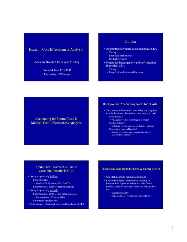
Outline
Issues in Cost-Effectiveness Analysis
Academy Health 2005 Annual Meeting
David Meltzer MD, PhD
University of Chicago
• Accounting for future costs in medical CEA
– Theory
– Empirical applications
– Productivity costs
• Preference heterogeneity and self-selection
in medical CEA
– Theory
– Empirical applications (Diabetes)
Background: Accounting for Future Costs
• Save patient with medical care today who requires
care in the future. Should we count that as a cost?
Accounting for Future Costs in
Medical Cost-Effectiveness Analysis
Traditional Treatment of Future
Costs and Benefits in CEA
• Analyses generally include:
– Future benefits
• Length of life/Quality of life = QALYs
– Future medical costs for related illnesses
• Analyses generally exclude:
– Future medical costs for unrelated illnesses
• Few exceptions: Weinstein, OTA
– Related illness?
• Angioplasty today, count bypass in future?
– Unrelated illness?
• Influenza vaccine today, count dialysis in future?
– Non-medical costs and benefits?
• Suicide prevention today, earnings in future?
Consumption in future?
Theoretical Background: Phelps & Garber (1997)
• Use lifetime utility maximization model
• Conclude: Obtain same relative rankings of
interventions if you include or exclude future
medical costs for unrelated illness as long as they
are:
• treated consistently
• truly unrelated = “conditional independence”
– Future non-medical costs
• Controversies reflect weak theoretical foundation of CEA
1
Intuition
Theoretical Background: Meltzer (1997)
• Consider two interventions with equal current cost
that both produce one QALY
• Use lifetime utility maximization model
• Conclude:
• A increases life expectancy by one year at QOL=1
• B increases life expectancy by two years at QOL=0.5
– Must include all future net resource use
• Medical costs - both related and unrelated - and future non-medical
costs net of earnings
• “Net resource use”= consumption + medical expenditures - earnings
• From -$10,000/ year @ age 25 to +$20,000/year @ age 85
• Which is preferred?
– From utility side: Indifferent
– From cost side: A preferred since it saves the costs of
supporting an extra year of life
– Hence, A preferred overall
– Relative rankings of interventions not independent of
future costs
• Analyses that omit future costs favor interventions that extend
life over those that improve quality of life
– Phelps/Garber inadvertently assume net annual
resource use is zero
• Omitting future costs favors interventions that
extend life (B) versus those that increase QOL (A)
Consumption, Medical Expenditure,
Earnings and Net Resource Use by Age
Accounting for Future Costs
Present Value of Future Net Resource
Use Per Year of Life Saved by Averting
Death (by Age)
30
20
Dollars (in thousands)
Δcost
Δpresent cost Δfuture cost
=
+
ΔQALY
ΔQALY
ΔQALY
Δpresent cost C * ΔLY
=
+
ΔQALY
ΔQALY
Δpresent cost
ΔLY
=
+ C*
ΔQALY
ΔQALY
10
Consumption
Medical Expenditure
Earnings
Net Resource Use
0
-10
-20
25
45
55
65
75
85
Age
Approximate Effects of Future Costs
Intervention
30
Dollars (thousands)
35
Cost/QALY
without
future costs
C
ΔLE/ΔQALY C∗(ΔLE/ΔQALY)
Cost/QALY
with
future costs
20
Treatment Severe
Hypertension
Men Age 40
$18,000
-$5,000
1.03
-$5,200
$12,800
10
Treatment Severe
Hypertension
Men Age 60
$60,000
$8,000
1.07
$8,500
$68,500
Adjuvant Chemo
Duke’s C Colon
CA Men Age 60
$67,000
$8,000
18
$144,000
$211,000
Hemodialysis for
ESRD
Men Age 60
$117,000
$8,000
1.5
$12,000
$129,000
0
-10
25
35
45
55
Age
65
75
85
2
So why not include future costs?
• Believe they belong, but don’t know how to
include them
• But methods are available:
• Believe they belong in theory, think it’s
“mean spirited”
• Meltzer JHE ‘97, Johannesson et al. MDM ‘97
• Can be as simple as including an age-specific
average net resource use
• Imprecise estimates better than zero
Effects of Future Costs for
Interventions among the Elderly
INTERVENTION
Hip Replacement
Women age 60
Hip Replacement
Men age 85
Treatment Mild HTN
Men age >70
Radiation Tx. MDPC
Age 65
ΔLY ΔQALY ΔLY/ΔQALY
So why not include future costs?
Δcost/ΔQALY
w/o future costs
Δcost/ΔQALY
w/ future costs
-0.03
6.9
-0.005
Cost-saving
Cost-saving
-0.02
2.0
-0.01
$9,177
$9,042
0.06
0.05
1.25
$5,000
$32,000
0.8
0.4
2
CECRC
CECRC+$32,000
Prostatectomy MDPC
0.7
0.2
3.5
CECRC
CECRC+$56,000
Age 65
HTN = Hypertension, MDPC = Moderately Differentiated Prostate Cancer
CECRC = Cost-effectiveness based on Current and Related Costs
– “Won’t this make it look like nothing is costeffective, don’t you believe in medicine?”
– “I have an 80 year-old father, the way I
understand your argument, you’re saying I
should kill him”
Effects of Future Costs for Interventions
among the Young and Elderly
Without Future
Costs
With Future
Costs
Cost-saving
Cost-saving
Treatment Mild HTN
Men Age>70
$5,000/QALY
$30,000/QALY
Hip Replacement
Men Age 85
$9,177/QALY
$9,042/QALY
Intensive Therapy IDDM
Starting Age 13-39
$30,000/QALY
$15,000/QALY
Hip Replacement
Women Age 60
So why not include future costs?
• Don’t believe they belong; think future costs
implicit in people’s answers to quality of life
questions
• However,
Do People Consider Financial
Factors in Answering Quality of
Life Questions?
– Costs due to increased life expectancy largely not borne
by individuals
– Empirical evidence that people do not consider these
costs when answering QALY questions
3
Background (continued)
Background
• Economic analysis of medical technology requires accurate
measurement of benefits and costs
– All relevant factors measured once and only once
– In accounting for future costs, this implies that lost
income should be counted as a cost
• Report of the Panel on Cost-effectiveness in Health and
Medicine argues that lost income should not be counted as
a cost in cost-effectiveness analysis
– Based on assumption that individuals consider income
changes when answering quality of life questions
– This has been used as an argument for excluding lost
income in accounting for future costs
• Active debate whether productivity costs are fully reflected in
QOL Measures (Brouwer et al. 1997, Meltzer and Johnanesson 1999)
– Discrepancies between personal and social costs
• public and private insurance
• payroll and income taxes
– Ambiguities about whether respondents consider personal
economic costs in answering QOL questions
• Health Utilities Index explicitly excludes lost income
• All other utility elicitation techniques silent on lost income
Effect of Economic Concerns on QOL Ratings
Objective
• To determine whether people consider financial factors in
answering quality of life questions
– Randomized subjects to versions of time trade-off
(TTO) questions that differ in guidance about
incorporating financial consequences of illness
– Asked patients whether they considered economic
factors when answering these questions
– Performed analyses for TTO questions concerning
blindness and back pain
Sample question: Which of the following would you prefer?
Live with blindness for 10 years.
Live in perfect health for 7 years.
No preference because these seem about the same.
QOL
(TTO)
No Guidance (NG)
4.95
-
Receive Disability (D)
4.83
P(D vs. NG) < N.S.
Not Receive Disability (ND)
4.84
P(ND vs. NG) < N.S.
Effect of Economic Concerns on QOL Ratings
Were People Thinking about Economic Concerns?
Sample question: Which of the following would you prefer?
Live with severe back pain for 10 years.
Live in perfect health for 7 years.
No preference because these seem about the same.
Question: When you answered this last set of questions,
were the possible financial effects of this back pain a
factor in your answer?
% Yes
QOL
(TTO)
No Guidance (NG)
5.09
-
Receive Disability (D)
5.78
P(D vs. NG) < 0.1
Not Receive Disability (ND)
4.24
P(ND vs. NG) < 0.03
No Guidance (NG)
13
-
Receive Disability (D)
20
P(D vs. NG) < 0.01
Not Receive Disability (ND)
21
P(ND vs. NG) < 0.01
4
Were People Thinking about Economic Concerns?
Question: When you answered these questions, were you
thinking about whether you would work?
Did Thinking about Financial Effects Change
TTO Values in the Absence of Guidance?
% Yes
No Guidance (NG)
24
-
Receive Disability (D)
31
P(D vs. NG) < 0.01
Not Receive Disability (ND)
40
P(ND vs. NG) < 0.01
QOL
(TTO)
Not Thinking about
Financial Effects
5.32
Thinking about Financial
Effects
4.15
P-value for
difference < 0.02
Conclusions
• Financial considerations may alter answers to TTO questions
– Average TTO values change with guidance about financial factors
– Standard TTO questions without guidance generate heterogeneous
assumptions across respondents
• Most people do not consider financial effects
• Respondents who consider financial effects give lower average
TTO values
Effects of Self-Selection on Cost-Effectiveness
• Even with guidance about financial factors, most respondents
say they were not a factor or that they were not thinking about
effects of illness on work
• Probably best to instruct people to ignore economic
consequences of illness and count those costs separately
Background
• Traditional CEA uses preferences (utilities) that average
across individuals
• However, utilities may vary across individuals or
populations and influence expected benefits of treatment
Standard CEA with Heterogeneous Individuals
CE
Δ costs
m
– Implies cost-effectiveness can vary for individuals or
populations that differ in preferences
• Preferences can also affect treatment choice
Δ effectiveness
– Specifically, patients whose preferences favor an option may
be more likely to choose it
• How might “self-selection” affect cost-effectiveness?
Blue Dots = Treated Patients
5
Perfect Self-Selection
Effect of Perfect Self-Selection on CEA
CE
Δ costs
m
CE
Δ costs
m
Δ effectiveness
Blue Dots=Pts gain from Tx; Orange Dots=Pts lose from Tx
Empirical Self-Selection
CE
Δ costs
m
Δ effectiveness
Blue Dots=Pts choose Tx; Orange Dots=Pts reject Tx
Methods: Interviews
• Interviewed 515 diabetes patients over age 65 attending
University of Chicago clinics from 1/1/01 to 1/1/2003
• Preferences (utilities) obtained by time trade-off questions
• Utilities obtained for
– Conventional and intensive glucose lowering (using
insulin or oral medications)
– Blindness, end-stage renal disease, lower extremity
amputation
• Data on treatment choices and patient characteristics
collected by medical records review
m’
Δ effectiveness
Blue Dots=Pts gain from Tx; Orange Dots=Pts lose from Tx (reject)
Background: Diabetes in the Elderly
• Diabetes care guidelines call for intensive lowering of
glucose among younger patients
• However, unclear if this should apply to older patients
– Gains in life expectancy smaller
– Side effects of treatment may dominate
– CE models of intensive therapy in older patients:
• Minimal or even negative effects on QALYs
• Not cost-effective
– Know many patients refuse intensive therapy
• Suggests self-selection may have important effects on
CEA in diabetes
Methods: Modeling
• NIH simulation model of intensive therapy for type 2 diabetes
(HbA1c 7% vs. 10%)
– Incorporated patient-specific data
• Age, sex, race, duration of diabetes
• Ran model using each individual’s utilities
– Intensive/conventional therapy, diabetic complications
• Analyses of cost-effectiveness of:
– Intensive vs. conventional therapy with insulin
– Intensive vs. conventional therapy with oral medications
• Contrast
– All patients vs. Perfect self-selection vs. Empirical selfselection
6
Results: Intensive Insulin Therapy vs.
Conventional Therapy
N
CE Approach
Group
Standard
Full Population
Results: Intensive Insulin Therapy vs.
Conventional Therapy
Change in Change in CE Ratio
Costs ($)
QALYs ($/QALY)
515
4826
-0.46
--
Perfect Self-Selection Effect for Intensive Insulin Therapy
N
CE Approach
Group
Change in Change in CE Ratio
Costs ($)
QALYs ($/QALY)
Standard
Full Population
515
4826
-0.46
--
Perfect SelfSelection
ΔQALY>0
309
4255
0.32
13K
ΔQALY<0
206
5682
-1.63
--
Empirical Self-Selection Effect for Intensive Insulin Therapy
20000
20000
CE
15000
15000
10000
10000
5000
5000
m
m’
0
0
-8
-6
-4
-2
0
2
4
-8
-6
-4
-2
0
2
4
-5000
-5000
Blue dots--the cost-effectiveness values of individuals with an expected benefit from intensive therapy.
Orange dots-- the cost-effectiveness values of individuals with a decrement in expected benefits with intensive therapy.
M-- CE ratio for whole population. M’—CE ratio after self-selection.
Results: Intensive Insulin Therapy vs.
Conventional Therapy
N
CE Approach
Group
Standard
Full Population
515
4826
Perfect SelfSelection
ΔQALY>0
309
ΔQALY<0
206
Self-identified
intensive
insulin therapy
All others
Empirical
Self-Selection
Blue dots-- cost-effectiveness values for individuals who identify their care as intensive therapy with insulin.
Orange dots-- cost-effectiveness values for all other individuals.
M-- CE ratio for orange dot individuals. M’-- CE ratio for blue dot individuals.
Results: Intensive vs. Conventional Oral Therapy
CE Approach Group
N
Change in Change in CE Ratio
Costs ($)
QALYs ($/QALY)
-0.46
--
4255
0.32
13K
5682
-1.63
--
97
2386
-0.03
--
418
5421
-0.56
--
Standard
Full Population
515
Change Change in CE Ratio
in Costs
QALYs ($/QALY)
($)
4826
0.17
28K
7
Results: Intensive vs. Conventional Oral Therapy
N
CE Approach Group
Change Change in CE Ratio
in Costs
QALYs ($/QALY)
($)
Results: Intensive vs. Conventional Oral Therapy
N
CE Approach Group
Change Change in CE Ratio
in Costs
QALYs ($/QALY)
($)
Standard
Full Population
515
4826
0.17
28K
Standard
Full Population
515
4826
0.17
28K
Perfect
Self-Selection
ΔQALY>0
427
4791
0.42
11K
Perfect
Self-Selection
ΔQALY>0
427
4791
0.42
11K
ΔQALY<0
88
4996
-1.04
--
ΔQALY<0
88
4996
-1.04
--
All
Oral Therapy
219
5892
0.06
104K
On Intensive
Oral Therapy
11
3294
0.29
11K
On Non-intensive
208
Oral Therapy
6029
0.04
136K
Empirical
Self-Selection
CDC-AAMC PEP Initial Results:
Intensive vs. Conventional Therapy
Limitations
• Modest sample size
• Limitations of the diabetes simulation model
N
CE Approach Group
– Model only compares HbA1c of 10% and 7%
– Does not model other diabetes-related treatments
Standard
Full Population
394
Change Change in CE Ratio
in Costs
QALYs ($/QALY)
($)
8007
-0.35
-
• Other definitions of intensive therapy
– E.g., actual treatments used, HbA1c
– Results stable with alternative definitions
• Unclear if utilities are valid or stable over time
– Might undermine predictive validity / welfare
interpretation
CDC-AAMC PEP Initial Results:
Intensive vs. Conventional Therapy
CE Approach Group
N
Implications
Change Change in CE Ratio
in Costs
QALYs ($/QALY)
($)
Standard
Full Population
394
8007
-0.35
-
Empirical
Self-Selection
On Intensive
Therapy
122
7777
0.18
43K
• Results of standard CEA may be misleading
– CEAs should consider the importance of selfselection
• Provides framework to value guidelines, decisionaids, or improved patient-doctor communication to
make care more consistent with patient preferences
• Suggests framework to design co-payment systems
to enhance cost-effectiveness of therapies
• Provides insight into policy making for voluntary
vs. involuntary interventions
8
Funding
• Centers for Disease Control and Prevention
– AAMC PEP (Meltzer, Huang)
– Center of Excellence in Health Promotion Economics
(Meltzer)
• National Institutes of Health
– NIDDK (Meltzer, Huang)
– NCI (R01 Meltzer)
• Robert Wood Johnson Foundation
– Generalist Physician Faculty Scholar Award (Meltzer)
Implications - I
Implications - II
• Results of standard CEA may be misleading
– In contrast to the suggestion of standard CEA, offering
intensive glucose lowering to all older people likely
cost-effective
– CEAs should consider the importance of selfselection
• Accounting for self-selection provides a
framework to value guidelines, decisionaids, or improved patient-doctor
communication that can make care more
consistent with patient preferences
• Distinction between perfect and empirical selfselection is potentially important
– Data on who will use a treatment if it is offered is
important
Motivation for Decision Aids
CE
Δ costs
m
Aim of Decision Aids
CE
Δ costs
m
Δ effectiveness
Blue Dots=Pts getting Tx; Orange Dots=Pts not getting Tx
Δ effectiveness
Blue Dots=Pts getting Tx; Orange Dots=Pts not getting Tx
9
Value of Decision Aids
CE
Δ costs
m
Δc
Δ effectiveness
Δe
Value of Decision Aid
• Effectiveness = ΣPts Δ Δe
• Costs = ΣPts Δ Δc
• Total Benefit
ΣPts Δ Δc
Cost-Benefit =
(1/λ) ΣPts Δ Δe +
Net Health Benefit =
ΣPts Δ Δe + λ ΣPts Δ Δc
Blue Dots=Pts getting Tx; Orange Dots=Pts not getting Tx
Implications - III
Motivation for Copayment
• Self-selection suggests a framework to design copayment systems to enhance the cost-effectiveness
of therapies
Δ costs
CE
m
Δ effectiveness
Blue Dots=Pts getting Tx; Orange Dots=Pts not getting Tx
Motivation for Copayment (πc)
πc
Δ costs
CE
Implications - IV
• Self-selection provides insight into policy making for voluntary
vs. involuntary interventions
– Voluntary: most medical interventions
• Self-selection improves value vs. population estimates
m
– Involuntary: environmental policy / safety regulation
• Population estimates more likely to be appropriate
Δ effectiveness
– Harms of pollution / safety risk non-selectively distributed
– Harms of regulation also non-selectively distributed
– Different standards for environmental regulation?
•
•
•
•
Traditionally high value of life -> low threshold for regulation
Reasonable if environmental harms not selectively avoidable
Not reasonable if harms of regulation also not selectively avoidable
Better approach: model selection and use common threshold
Blue Dots=Pts getting Tx; Orange Dots=Pts not getting Tx
10
Funding
• Centers for Disease Control and Prevention
– AAMC PEP (Meltzer, Huang)
– Center of Excellence in Health Promotion Economics
(Meltzer)
• National Institutes of Health
– NIDDK (Meltzer, Huang)
– NCI (R01 Meltzer)
• Robert Wood Johnson Foundation
– Generalist Physician Faculty Scholar Award (Meltzer)
Specific Aims
Effects of Quality of Life
on the Cost-Effectiveness
of Prostate Cancer Treatment
David O. Meltzer, MD, PhD
Anirban Basu, MS
Brian L. Egleston, MPP
Qi Zhang, PhD
Background on Prostate Cancer
• Most commonly diagnosed non-cutaneous cancer, among
US men
• Second most common cause of cancer-related death among
US men
• To develop a sophisticated decision-analytic
model to evaluate cost, effects, and costeffectiveness alternative treatments for clinically
localized prostate cancer by age and tumor grade
• To assess how the cost-effectiveness of prostate
cancer treatments will be affected by including
possible effects of anxiety on QOL
• To assess how patient self-selection might affect
the cost-effectiveness of treatment
Challenges
• PC screening and treatment remains controversial
• Effects on mortality unclear
– Little clear evidence from randomized trials
– Mortality trends post screening not established
• Presence of significant morbidities associated with treatment
• 198,100 new cases diagnosed and 31,500 deaths in 2001
• Significant variation in outcomes by tumor grade, patient age
• ~80% of clinically diagnosed PC in men 65+
• Significant costs of screening and treatment of localized PC
• Because older persons have high competing risks of death,
many men die with prostate cancer rather than of it.
• Cost-effectiveness studies of treatment differ in findings
• <10% men with PC die of it within 5 years of diagnosis
• Cost-effectiveness studies of screening differ even more greatly
– Increase QALYs (Kattan)
– Increase survival but not QALYs (Fleming)
11
Flaws in Published Models
• Failure to model PC incidence as a dynamic process affected by
previous screening through effects on prevalence of latent disease
• Failure to distinguish between cancers of differing stage and grades
(heterogeneity)
• Model progression based on clinical rather than pathological stage, or
without any empirical basis
• Many models are of one-time screen (exception: Etzioni et. al. 1999)
• Other problems:
– Confuse PPV/NPV of screening tests vs. sensitivity/specificity,
– Failure to model QOL and/or cost,
– Other technical and data related issues.
Key Features of Our Model
vs. Published Models
Prostate Cancer Model: Overview
• Development of Model Structure
– Natural history model
– Detection model
• Parameter Estimation
–
–
–
–
–
Literature review
Secondary data analysis
Mathematical modeling
Fitting to aggregate incidence, prevalence, & mortality by age
Maximum likelihood estimation
• Cancer stage and grade transitions
• Mortality rates from metastatic disease
• Estimation of Cost-Effectiveness of:
• Screening policies
• Treatment policies
The Model
• Markov model of screening and treatment
– Annual cycles from age 50 to 99
• Tumor heterogeneity and progression rates by grade
• Misclassification of tumor stage due to the discrepancy
between clinical and pathologic stage
• The ability of screening and treatment to affect the
prevalence of prostate cancer in the undetected population
• The effect of benign prostatic hypertrophy and its
management on the detection of prostate cancer
• The potential effects of screening and treatment on quality
of life, as measured by quality-adjusted life expectancy
Model Structure: Overview
• Natural history model including stage and grade
– Possibility of early metastases
• Repeat screening requires treating many factors as
state variables
– Even small rates lead to 100% intervention rates over time
– We created a state vector with 1,440 states
BPH symptoms
PSA/Rectal detectable
History of screening
Presence of metastases
Metastatic detectable
History of TURP
Local cancer stage
Local grade
Model Structure: Natural History
N A B C D
Initial Stage Distribution
Well
Moderate
Poor
No Cancer
N A B C D
Detection
Non-Detected
Population
Transition Probabilities
N A B C D
Incidence Rate
Cured
N A B C D
Death from
Other Causes
Not Cured
N A B C D
Death from Prostate Cancer
or Other Causes
N A B C D
Local Stage A
Local Stage B
Local Stage C
Transition Probabilities
Death from Prostate Cancer
or Other Causes
Non-metastatic disease
Metastatic disease
12
Model Structure: Detection
Symp = Symptoms
Mot = Motivated
Pos = Positive
Neg = Negative
TURP = Transurethral Resection
of the Prostate
MWU = Metastatic Work-up
Palp Ext = Palpable Extension
Clin = Clinical Stage
Comp = Complications
Model Structure: State Variables
– Pathologic Stage
• Local stage (no cancer, A, B, C)
• Presence of metastases (D)
– Grade
• Well, moderate, poor
– Presence of BPH symptoms
– Presence of cancer symptoms
– History of TURP for BPH symptoms
– Cancer detectability
• Digital rectal exam and/or PSA detectability
– History of regular prostate cancer screening
Parameter Estimation: Direct Approaches
Parameter
Derivation Technique
Primary References
P(Symptom Motivated Exam)
Literature Review
Meigs et al., 1998
P(Biopsy | Positive Exam)
Secondary Data Analysis
Richie et al., 1993
P(Biopsy Positive | Pathologic Stage)
Geometric Prostate Model
McNeal et al., 1986
Catalona et al., 1996
Lu-Yao et al., 1996
Parameter Estimation: Direct Approaches
Parameter
Derivation Technique
P(Prostate Cancer | Age)
Meta-Analysis
Multiple sources
P(DRE or PSA Detectable Prostate Cancer)
Maximum Likelihood
Estimation and
Secondary Data Analysis
Literature Review
Richie et al., 1993
P(Metastatic Work-Up Positive)
Mathematical Modeling
P(Clinical Stage | Pathologic Stage)
Secondary Data Analysis
SEER data
P(Symptomatic BPH)
P(Treatment | Clinical Stage)
Secondary Data Analysis
SEER data
P(Symptoms | Prostate Cancer)
P(Complications | Treatment)
Literature Review
Wasson et al., 1993
P(Cure Rates | Treatment and Pathologic Stage)
Literature Review and
Model Assumptions
D’Amico et al., 1998
P(Transurethral Resection of the Prostate [TURP])
Secondary Data Analysis
P(Postive Pathologic Findings | TURP)
Literature Review and
Mathematical Analysis
National Hospital
Discharge Survey
National Survey of
Ambulatory Data
Coffield et al., 1992
Babaian et al., 1991
P(Routine Screening Exam for Prostate Cancer)
Literature Review
Meigs et al., 1998
P(History of Prostate Cancer Screening)
Literature Review
Meigs et al. 1998
Model Validation and
Indirect Parameter Estimation
Relationship between grade and stage
Mathematical Modeling
Literature Review
Literature Review
Primary References
Meigs et al., 1998
Multiple Sources
Middleton et al., 1988
Prostate Cancer Related Mortality
Data Analysis
SEER Data
Age-Specific All-Cause Mortality
Literature Review
Quality of Life
Literature Review
Social Security
Administration
Multiple Sources
Model Fit
• Curve fitting
– Aggregate SEER incidence and mortality data
• Maximum likelihood estimation
– Individual level SEER-Medicare data
• Stage-treatment-age
• Outcomes (mortality, metastatic disease)
• e.g. P(die PC age 76| T1a, RPx, 68)
13
Cost-Effectiveness of Treatment
Baseline Analysis (Age 55 yrs)
Individual Fitting: SEER vs. Life Table Data
Age (years), and
Well Differentiated
Outcome
WW
Age
SEER
PC Mort
3.58%
2.07%
1.38%
1.71%
1.25%
55
65
75
85
95
SEER
Non-PC Mort
0.36%
2.03%
2.72%
3.72%
2.92%
Life Table
Non-PC Mort
0.89%
2.23%
4.86%
11.82%
26.15%
RP
RT
Moderately
Differentiated
WW
RP
RT
Poorly Differentiated
WW
RP
RT
55
+
Expected Costs
Non-Discounted LYs
+
Discounted LYs
+
Discounted QALYs
5483
34515 35125
6463
27630 28106
8047
23435 23815
21.82
22.53
22.64
19.88
21.61
21.71
16.48
19.21
19.3
13.39
13.63
13.69
12.49
13.18
13.24
10.75
11.93
11.98
13.32
9.84
11.45
12.28
9.48
11.02
10.38
8.52
9.89
+ Discount Rate of 3% is used, Costs is 1993 $. QOL weight for Impotence, Incontinence, Bowel Dysfunction, Urethral
Stricture and Metastasis are added.
Cost-Effectiveness of Treatment
Cost-Effectiveness of Treatment
Baseline Analysis (Age 65 yrs)
Baseline Analysis (Age 75 yrs)
Age (years), and
Well Differentiated
Outcome
WW
RP
RT
Moderately
Differentiated
WW
RP
RT
Age (years), and
Poorly Differentiated
Well Differentiated
Outcome
WW
RP
RT
Moderately
Differentiated
Poorly Differentiated
WW
RP
RT
WW
RP
RT
WW
RP
RT
75
65
+
+
Expected Costs
5993
39044 39733
4784
20181 20527
5646
12613
12795
Expected Costs
4612
31935
32502
3320
17389
17689
2466
6255
6315
Non-Discounted LYs
14.83
15.17
15.25
13.53
14.46
14.53
10.85
11.78
11.84
Non-Discounted LYs
9.24
9.26
9.32
8.71
8.85
8.9
7.15
7.24
7.28
7.41
7.52
7.56
6.91
7.23
7.27
5.73
6.08
6.11
Discounted LYs
3.73
3.73
3.75
2.39
2.39
2.4
2.99
3.01
3.03
3.71
2.69
3.13
3.48
2.57
2.99
2.80
2.09
2.41
+
Discounted LYs
+
Discounted QALYs
7.37
5.43
6.32
6.76
5.19
6.04
5.43
4.28
+ Discount Rate of 3% is used, Costs is 1993 $. QOL weight for Impotence, Incontinence, Bowel Dysfunction, Urethral
Stricture and Metastasis are added.
Two-way Sensitivity Analysis of Cost-Effectiveness with
Impotence & Incontinence QOL (Age 55 yrs)
4.95
+
+
Discounted QALYs
+ Discount Rate of 3% is used, Costs is 1993 $. QOL weight for Impotence, Incontinence, Bowel Dysfunction, Urethral
Stricture and Metastasis are added.
Psychological Anxiety
• Patients with known prostate cancer may have anxiety that
affects QOL.
QOL of Patients detected with prostate cancer = Anxiety QOL
(if no other side effects)
• Anxiety may be reduced with treatment
With Surgery:
If Cured: Patient’s QOL =1.0
(i.e. Confirmed Elimination of PC related Anxiety)
If not cured: Patient's QOL = Anxiety QOL
With Radiation:
If Cured: Patient’s QOL = (1+ Anxiety QOL)/2
(i.e. Unconfirmed Elimination of PC related Anxiety)
If not cured: Patient's QOL = Anxiety QOL
14
Moderately Differentiated
Poorly Differentiated
Age 55
Age 55
W
QALYs
QALYs
W
R
R
6
4
2
0
0.6
0.7
0.8
0.9
1
W
12
W
R
R
R
10
R
R
R
8
7
6
5
4
3
2
1
0
R
W
8
6
4
2
0
0.6 0.7 0.8 0.9
0.6 0.7
1
0.8 0.9
W
R
R
W
0.7
0.8
0.9
Anxiety QOL
* Letter above bar indicates most beneficial treatment that is
cost-effective (<$100K/QALY)
Poorly Differentiated
Age 65
Age 65
W
0.6
1
Anxiety QOL
Anxiety QOL
Anxiety QOL
Moderately Differentiated
Age 65
14
QALYs
14
12
10
8
14
12
10
8
6
4
2
0
W
Well Differentiated
QALYs
Age 55
QALYs
Well Differentiated
One-way Sensitivity Analysis of Anxiety QOL on
Baseline Estimates (Age 65 yrs)
1
8
7
6
5
4
3
2
1
0
W
R
R
R
W
0.6 0.7 0.8 0.9
Anxiety QOL
QALYs
One-way Sensitivity Analysis of Anxiety QOL on
Baseline Estimates (Age 55 yrs)
1
8
7
6
5
4
3
2
1
0
R
R
R
0.6
0.7
0.8
W
0.9
W
1
Anxie ty QOL
* Letter above bar indicates most beneficial treatment that is
cost-effective (<$100K/QALY)
CEA Phase Diagrams with Anxiety, Impotence and Incontinence QOL for Age = 55 yrs
One-way Sensitivity Analysis of Anxiety QOL on
Benefits and Cost-Effectiveness (Age 75 yrs)
Well Differentiated
Moderately Differentiated
W
W
R
W
Age 75
W
0.6 0.7 0.8 0.9
Anxiety QOL
1
4
3.5
3
2.5
2
1.5
1
0.5
0
W
R
R
W
W
QALYs
4
3.5
3
2.5
2
1.5
1
0.5
0
1.0
Poorly Differentiated
Age 75
QALYs
QALYs
Age 75
Anxiety QOL
0.6 0.7 0.8 0.9
1
4
3.5
3
2.5
2
1.5
1
0.5
0
W
R
R
W
W
0.8
0.6 0.7
Anxiety QOL
0.8 0.9
1
Anxiety QOL
0.6
* Letter above bar indicates most beneficial treatment that is
cost-effective (<$100K/QALY)
CEA Phase Diagrams with Anxiety, Impotence and Incontinence QOL for Age = 65 yrs
CEA Phase Diagrams with Anxiety, Impotence and Incontinence QOL for Age = 75 yrs
Anxiety QOL
Anxiety QOL
1.0
1.0
0.8
0.8
0.6
0.6
15
RESULTS
• Treatments cost-effective vs. watchful-waiting only at
high QOL of impotence and incontinence and younger
ages.
• Radiation tends to be cost-effective than surgery
• Results not sensitive to bowel dysfunction and metastasis
QOL
• Results very sensitive to anxiety QOL.
– Anxiety QOL=0.8 makes radiation cost-effective even
at low QOL of other complication.
• Patient preferences important determinant of optimal care
• Self-selection may be a critical determinant of costeffectiveness
Panel’s Position on Morbidity Costs
• Effects on income and leisure should be excluded
from costs since included in QALY weights
– Assume people take private economic effects
into account in answering QOL questions
– Exception: effects of lost productivity borne by
others (e.g. “friction costs” borne by employees
and coworkers)
Problems with Panel’s Position on
Morbidity Costs
• Inappropriate exclusion of lost earnings not
reflected in private costs
• Disability insurance (public or private)
• Taxes (employee and employer)
• Inappropriate inclusion of costs already reflected
in private costs
• Out-of-pocket health care costs
• Time costs in chronic illness (e.g. ESRD)
Conclusions
• Financial considerations may alter answers to TTO questions
– Average TTO values change with guidance about financial factors
– Standard TTO questions without guidance generate heterogeneous
assumptions across respondents
• Most people do not consider financial effects
• Respondents who consider financial effects give lower average
TTO values
• Even with guidance about financial factors, most respondents
say they were not a factor or that they were not thinking about
effects of illness on work
• Probably best to instruct people to ignore economic
consequences of illness and count those costs separately
– But further study is needed
16
Cost-Effectiveness of Pap Smears
Increase in
LE
vs. no
screening
Cost
vs. no
screening
Average
Cost per
Life-Yr
Saved
Marginal
increase in
Cost
Marginal
Increase in
Cost
Marginal
Cost per
Life-Yr
Saved
3 years
70 days
$100
$521/LY
70 days
$100
$521/LY
2 years
71 days
$150
$771/LY
1 day
$50
$18,250
/LY
1 year
71 days
8 hours
$300
$1,535/LY
8 hours
$150
$165,909
/LY
Frequency
Why the difference versus
Phelps and Garber?
• In some models, they assume consumption =
production in every period
– This sets future costs = 0
• In others, they incorrectly apply an equilibrium
condition from a model without future costs to a
model that includes future costs
– This holds in the future costs model only if
future costs = 0
Limitations
• Estimates of future costs may be imprecise
– Prostate cancer estimates based on ΔLY/ΔQALY
• Ideally, costs should be included directly in the decision model
– Future consumption, medical expenditures and earnings
may be hard to predict. However:
• Imprecise estimates are presumably better than implicit
estimate of zero
• Sensitivity analyses can and should be performed
• This should include estimates that exclude future costs
– Reflection of resource costs in QALYs not clear
• Especially non-market consumption and production
• This is an issue for current costs as well
QALYs
• Total years lived with each year weighted
between 0 and 1
– Death: 0
– Perfect health: 1
• QALYs = Σ tStQt
– St survival probability
– Qt quality of life adjustment
–
< 1 time preference discount factor
Limitations
• Estimates of future costs may be imprecise
– Prostate cancer estimates based on ΔLY/ΔQALY
• Ideally, costs should be included directly in the decision model
– Future consumption, medical expenditures and earnings
may be hard to predict. However:
• Imprecise estimates are presumably better than implicit
estimate of zero
• Sensitivity analyses can and should be performed
• This should include estimates that exclude future costs
– Reflection of resource costs in QALYs not clear
• Especially non-market consumption and production
• This is an issue for current costs as well
Methods
• Study Population
– 831 adults interviewed while waiting for scheduled physician
visits in an academic primary care practice
– Separate surveys for blindness (N=429) and back pain (N=402)
– Ages 18-65
• Survey Design
– Description of health states
• “permanent blindness”
• “severe chronic back pain that occurs every day for at least half the day”
• No explicit mention of effects on work in health state description
– Subjects then asked time trade-off question in one of three
randomly assigned forms:
17
TTO Versions
Version 0: “Imagine you have developed severe chronic back
pain and have 10 years to live.”
Version 1: Version 0 + “Depending on your occupation and
personal choice, this might or might not prevent you from
working. If you were unable to work, I would like you to
assume that you would receive disability payments equal to
60% of your current income”
Version 2: Version 0 + “Depending on your occupation and
personal choice, this might or might not prevent you from
working. If you were unable to work, I would like you to
assume that you would receive no disability payments.”
Methods: Follow-up Questions
• “When you answered this last set of questions, were the
possible financial effects of this illness a factor in your
answer?”
• “Were you thinking about whether you would work?”
• Beliefs about effects of the illness on employment status
and income
• Demographic information, current employment status, and
income
Results: Population Characteristics
Age (years)
Mean (SD)
Race
Black
White
Other
Job Status
Working
Retired
Student
Homemaker
Disabled
Unemployed
Other
Household Income
< $25,000
$25,000 - $50,000
>$50,000
Overview
39 (14)
52%
34%
14%
63%
14%
10%
3%
3%
3%
5%
• Theory of self-selection
• Initial results on self-selection in diabetes
treatment
• Prostate cancer model and likely importance
of self-selection
28%
34%
38%
Overall Aim and Hypotheses
• Overall Aim: To evaluate the impact of self-selection on
the cost-effectiveness of intensive glucose lowering
therapy among older patients with diabetes
Results: Patient Characteristics (N=515)
Mean Age,
years (Std. Deviation (SD))
Female, %
74 (5.9)
63
Ethnicity
• H1: Perfect self-selection will make intensive therapy
more cost-effective compared to its cost-effectiveness in
the full population of older patients with diabetes
African American, %
Caucasian, %
Hispanic, %
• H2: Empirical self-selection will make intensive therapy
more cost-effective compared to its cost-effectiveness in
the full population of older patients with diabetes
Asian, %
Mean duration of Diabetes,
years (SD)
79
16
2.5
0.4
13 (10)
18
Results: Complication Health State Utilities
Results: Treatment Health State Utilities
Health State
Mean (95% CI)
Health State
Mean (95% CI)
Blindness
0.39 (0.36-0.42)
Conventional glucose lowering
0.76 (0.73-0.78)
End-stage renal disease
0.36 (0.34-0.39)
0.77 (0.75-0.80)
Lower extremity amputation
0.45 (0.42-0.48)
Intensive glucose lowering with
oral medications
Intensive glucose lowering with
insulin
0.64 (0.61-0.67)
Results: Effects of Future Costs for
Interventions among the Young
Without Future
Costs
With Future
Costs
Intensive Therapy IDDM
(Meltzer et al. 1999)
$48,000/LY
$23,000/LY
Intensive Therapy IDDM
(Meltzer et al. 1999)
$30,000/QALY
$15,000/QALY
HAART – base case
(Sendi et al., 1999)
$22,000/LY
Cost-saving
HAART – pessimistic case
(Sendi et al., 1999)
$30,000/LY
$4,000/LY
19