STAT 495, Fall 2003
Homework Assignment #3
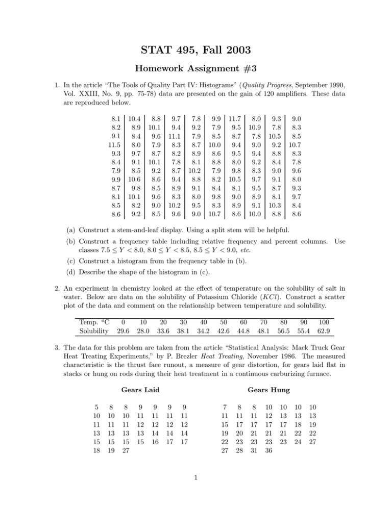
1. In the article “The Tools of Quality Part IV: Histograms” (Quality Progress, September 1990,
Vol. XXIII, No. 9, pp. 75-78) data are presented on the gain of 120 amplifiers. These data
are reproduced below.
8.1
8.2
9.1
11.5
9.3
8.4
7.9
9.9
8.7
8.1
8.5
8.6
10.4
8.9
8.4
8.0
9.7
9.1
8.5
10.6
9.8
10.1
8.2
9.2
8.8
10.1
9.6
7.9
8.7
10.1
9.2
8.6
8.5
9.6
9.0
8.5
9.7
9.4
11.1
8.3
8.2
7.8
8.7
9.4
8.9
8.3
10.2
9.6
7.8
9.2
7.9
8.7
8.9
8.1
10.2
8.8
9.1
8.0
9.5
9.0
9.9
7.9
8.5
10.0
8.6
8.8
7.9
8.2
8.4
9.8
8.3
10.7
11.7
9.5
8.7
9.4
9.5
8.0
9.8
10.5
8.1
9.0
8.9
8.6
8.0
10.9
7.8
9.0
9.4
9.2
8.3
9.7
9.5
8.9
9.1
10.0
9.3
7.8
10.5
9.2
8.8
8.4
9.0
9.1
8.7
8.1
10.3
8.8
9.0
8.3
8.5
10.7
8.3
7.8
9.6
8.0
9.3
9.7
8.4
8.6
(a) Construct a stem-and-leaf display. Using a split stem will be helpful.
(b) Construct a frequency table including relative frequency and percent columns. Use
classes 7.5 ≤ Y < 8.0, 8.0 ≤ Y < 8.5, 8.5 ≤ Y < 9.0, etc.
(c) Construct a histogram from the frequency table in (b).
(d) Describe the shape of the histogram in (c).
2. An experiment in chemistry looked at the effect of temperature on the solubility of salt in
water. Below are data on the solubility of Potassium Chloride (KCl). Construct a scatter
plot of the data and comment on the relationship between temperature and solubility.
Temp. o C
Solubility
0
29.6
10
28.0
20
33.6
30
38.1
40
34.2
50
42.6
60
44.8
70
48.1
80
56.5
90
55.4
100
62.9
3. The data for this problem are taken from the article “Statistical Analysis: Mack Truck Gear
Heat Treating Experiments,” by P. Brezler Heat Treating, November 1986. The measured
characteristic is the thrust face runout, a measure of gear distortion, for gears laid flat in
stacks or hung on rods during their heat treatment in a continuous carburizing furnace.
Gears Laid
5
10
11
13
15
18
8
10
11
13
15
19
8
10
11
13
15
27
9
11
12
13
15
9
11
12
14
16
Gears Hung
9
11
12
14
17
9
11
12
14
17
7
11
15
19
22
27
1
8
11
17
20
23
28
8
11
17
21
23
31
10
12
17
21
23
36
10
13
17
21
23
10
13
18
22
24
10
13
19
22
27
(a) Construct a histogram for all 77 gears using intervals: 5 ≤ Y < 10, 10 ≤ Y < 15,
15 ≤ Y < 20, etc.
(b) Construct separate histograms for the gears hung and the gears laid using the same
intervals as in (a). Compare the two methods of handling gears. How do the handling
methods differ in terms of runout measurements?
4. The data for the following problem come courtesy of Steve Vardeman at Iowa State University. A gauge R&R study was conducted using 2 sheets of paper (Part) and 5 operators. Each
sheet of paper was weighed three times by each operator. All measurements were made using
the same scale.
1
1
3.481
3.477
3.470
2
3.480
3.472
3.470
3.259
3.254
3.258
3.254
3.247
3.249
Operator
3
4
3.485 3.470
3.475 3.468
3.477 3.463
5
3.472
3.470
3.474
Part
2
3.256
3.258
3.245
3.253
3.242
3.246
3.241
3.249
3.254
(a) Using the method presented in lecture/tape 8, compute the estimate of σ Repeat and the
estimate of σReprod . Give the percentage of variation due to the gauge and that due to
the operator. Where should improvement efforts be focused - training the operators or
purchasing new gauges?
(b) Use JMP to compute variance components for these data. How do the percentages for
gauge and operator compare to those in part (a)? Including the parts, how much of the
total variation is due to the measurement system?
2