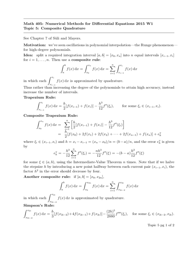
Math 405: Numerical Methods for Differential Equations 2015 W1
Topic 5: Composite Quadrature
See Chapter 7 of Süli and Mayers.
Motivation: we’ve seen oscillations in polynomial interpolation—the Runge phenomenon—
for high-degree polynomials.
Idea: split a required integration interval [a, b] = [x0 , xn ] into n equal intervals [xi−1 , xi ]
for i = 1, . . . , n. Then use a composite rule:
Z xn
Z b
n Z xi
X
f (x) dx =
f (x) dx
f (x) dx =
a
Z
x0
i=1
xi−1
xi
in which each
f (x) dx is approximated by quadrature.
xi−1
Thus rather than increasing the degree of the polynomials to attain high accuracy, instead
increase the number of intervals.
Trapezium Rule:
Z xi
h
h3 00
f (x) dx = [f (xi−1 ) + f (xi )] − f (ξi ),
2
12
xi−1
for some ξi ∈ (xi−1 , xi ).
Composite Trapezium Rule:
Z xn
n X
h
h3 00
f (x) dx =
[f (xi−1 ) + f (xi )] − f (ξi )
2
12
x0
i=1
h
=
[f (x0 ) + 2f (x1 ) + 2f (x2 ) + · · · + 2f (xn−1 ) + f (xn )] + eTh
2
where ξi ∈ (xi−1 , xi ) and h = xi − xi−1 = (xn − x0 )/n = (b − a)/n, and the error eTh is given
by
n
h3 X 00
nh3 00
h2
T
eh = −
f (ξi ) = −
f (ξ) = −(b − a) f 00 (ξ)
12 i=1
12
12
for some ξ ∈ (a, b), using the Intermediate-Value Theorem n times. Note that if we halve
the stepsize h by introducing a new point halfway between each current pair (xi−1 , xi ), the
factor h2 in the error should decrease by four.
Another composite rule: if [a, b] = [x0 , x2n ],
Z b
Z x2n
n Z
X
f (x) dx =
f (x) dx =
a
Z
x0
i=1
x2i
f (x) dx
x2i−2
x2i
in which each
f (x) dx is approximated by quadrature.
x2i−2
Simpson’s Rule:
Z x2i
(2h)5 0000
h
f (ξi ),
f (x) dx = [f (x2i−2 )+4f (x2i−1 )+f (x2i )]−
3
2880
x2i−2
for some ξi ∈ (x2i−2 , x2i ).
Topic 5 pg 1 of 2
Composite Simpson’s Rule:
Z x2n
n X
h
(2h)5 0000
f (x) dx =
[f (x2i−2 ) + 4f (x2i−1 ) + f (x2i )] −
f (ξi )
3
2880
x0
i=1
h
[f (x0 ) + 4f (x1 ) + 2f (x2 ) + 4f (x3 ) + 2f (x4 ) + · · ·
=
3
+ 2f (x2n−2 ) + 4f (x2n−1 ) + f (x2n )] + eSh
where ξi ∈ (x2i−2 , x2i ) and h = xi − xi−1 = (x2n − x0 )/2n = (b − a)/2n, and the error eSh is
given by
n
(2h)5 X 0000
n(2h)5 0000
h4 0000
S
eh = −
f (ξi ) = −
f (ξ) = −(b − a)
f (ξ)
2880 i=1
2880
180
for some ξ ∈ (a, b), using the Intermediate-Value Theorem n times. Note that if we halve
the stepsize h by introducing a new point half way between each current pair (xi−1 , xi ),
the factor h4 in the error should decrease by sixteen (assuming f is smooth enough).
Adaptive (or automatic) procedure: if Sh is the value given by Simpson’s rule with
a stepsize h, then
15
Sh − S 1 h ≈ − eSh .
2
16
Z b
This suggests that if we wish to compute
f (x) dx with an absolute error ε, we should
a
compute the sequence Sh , S 1 h , S 1 h , . . . and stop when the difference, in absolute value,
2
4
between two consecutive values is smaller than 16
ε. That will ensure that (approximately)
15
S
|eh | ≤ ε.
Often spatially-varying adaptivity is used in practice: refine only is regions where a
local estimate is large.
Comments:
Sometimes much better accuracy may be obtained: for example, as might happen when
computing Fourier coefficients, if f is periodic with period b − a so that f (a + x) = f (b + x)
for all x.
Topic 5 pg 2 of 2