APPENDIX - Analysis of variance and associated statistical calculations
This appendix presents mathematical equations for the statistical models described in the
guidelines. They pertain specifically to quantitative and semi-quantitative disinfectant tests. The
formulae use the terminology of Table 1 and notation of Table 2.
Two alternative statistical techniques are commonly used for estimating the variances for
the random effects in these ANOVA models, the method of moments (MOM) and the restricted
maximum likelihood (REML) method. The MOM is recommended for balanced data and the
REML method is recommended for unbalanced data; e.g., (1) in which the MOM is called the
ANOVA method. When there is mild imbalance or the unbalanced design possesses certain
regularities, either technique is acceptable.
A. One-factor, random effects model for LR values
This model underlies the ANOVA for repeatability and reproducibility assessments (3)
and for responsiveness assessments. Let LRim denote the LR for the mth replicate of the test in the
ith laboratory. The one-factor, random effects model submitted to ANOVA is:
LRim = µ + βi + εim,
where µ is the true mean LR, βi is the random effect due to the ith laboratory, and εim is the
random effect due to the mth replicate test in the ith laboratory. The analysis requires that βi and
εim, for all i and m, are independent random variables having means of zero. The estimated
variance of βi is the variance among laboratories, S2lab, and the estimated variance of εim is the
repeatability variance within a laboratory, Sr2. This model assumes that the true repeatability
variance is homogeneous across laboratories.
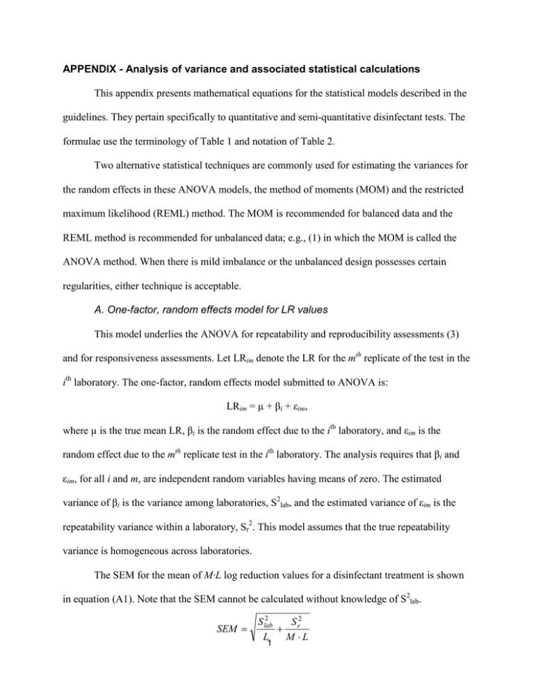
The SEM for the mean of M·L log reduction values for a disinfectant treatment is shown
in equation (A1). Note that the SEM cannot be calculated without knowledge of S2lab.
SEM =
2
S lab
S2
+ r
L
M ⋅L
1
(A1)
B. Nested 2-factors random effects model for LD values
This model underlies the ANOVA for resemblance assessment. Let LDimj denote the log
density for the jth untreated carrier in the mth replicate of the test in the ith laboratory. The 2factors, nested random effects statistical model submitted to ANOVA is:
LDimj = µ + βi + γm(i) + εimj,
where µ is the true mean LD, βi is the random effect due to the ith laboratory, γm(i) is the nested
random effect due to the mth replicate test in the ith laboratory, and εimj is the nested random effect
due to the jth carrier in the mth replicate test in the ith laboratory. The analysis requires that βi,
γm(i), and εimj, for all i, m, and j, are independent random variables having means of zero. The
estimated variance of βi is the variance among laboratories (US2lab), the estimated variance of
γm(i) is the variance among replicate tests within a laboratory (US2test), and the estimated variance
of εimj is the variance among untreated carriers within a test (US2). The estimate of µ is the
overall mean log density for untreated carriers. This model assumes that the true within-test
variance is homogeneous across all tests and the true variance among tests within a laboratory is
homogeneous across laboratories.
C. Example: ANOVA and associated calculations using the statistical
programming language R
Tables 3-5 of this manuscript provide results of the resemblance, repeatability,
reproducibility, and responsiveness analyses of data presented in (16) for an 8-lab study of the
Three Step Method (TSM). This appendix shows the computer code for calculating those results
using the package nlme (2) within R (3); R is a free software environment for statistical
computing and graphics.
2
In R programming, the symbol > is a prompt for the next command and the symbol #
indicates a comment that is not an executable command. All files created here should be located
in the R working directory on your computer. The computer code and corresponding output are
in this typeface. Output lines will not be preceded by the prompt (>).
R commands: resemblance analysis
To import the TSM untreated carrier LD values into R, first copy and paste the control
data from Appendix B of (16) into a tab-delimited text file called
ControlDataFromTomasino2008.txt. Edit that text file so the first row contains the column labels
(Lab Test LD) separated by tabs. Then those control data can be imported into the R as a data
object called d.control via the read.table command.
> # Read in a tab delimited text file of the control data
> d.control = read.table("ControlDataFromTomasino2008.txt",header=T)
List the data to check that it was properly imported; because of space limitations here, we only
list the first 9 lines. Note that the first column in the list was added by R to show what rows of
the data matrix were listed.
> # Look at the 1st 9 lines of data
> d.control[1:9,]
Lab Test
LD
1
1
1 6.916262
2
1
1 6.848245
3
1
1 6.993236
4
1
2 6.712650
5
1
2 6.754626
6
1
2 6.793854
7
1
3 6.738492
8
1
3 6.820560
9
1
3 6.938156
The 2-factors, nested random effects ANOVA, based on the model of Appendix B, is fit to the
control LDs as follows.
> # Load the nlme package into R
> library(nlme)
3
>
>
>
>
# Fit a nested 2-factors, random effects ANOVA model
m.control = lme(LD ~ 1,random=~1|Lab/Test, data=d.control)
# Display the results
summary(m.control)
Linear mixed-effects model fit by REML
Data: d.control
AIC
BIC
logLik
-101.6162 -88.13363 54.80809
Random effects:
Formula: ~1 | Lab
(Intercept)
StdDev:
0.2213407
Formula: ~1 | Test %in% Lab
(Intercept) Residual
StdDev:
0.1267794 0.1448101
Fixed effects: LD ~ 1
Value Std.Error DF t-value p-value
(Intercept) 6.862976 0.0802763 144 85.49194
0
> # Ignore the DF and p-value outputted by R
The above R output after “Random effects:” is easily converted to the variances
presented in Table 4(a) by squaring the SDs: US2lab = 0.22134072 = 0.04899, US2test =
0.12677942 = 0.01607, and US2 = 0.14481012 = 0.02097. The output after “Fixed effects:”
shows that the overall mean of TestLDs is 6.862976 and the SEM is 0.0802763. The
repeatability SD, reproducibility SD, and SEM can be calculated via equations (6),(7) and (8)
respectively by the following R code (cf. Table 4(b)).
> varLD.output=VarCorr(m.control)
> varLD = as.numeric(varLD.output[c(2,4,5),1])
> US2 = varLD[3]
> US2_test= varLD[2]
> US2_lab = varLD[1]
> L = m.control$dims$ngrps[2]
# L = 8 labs
> M = m.control$dims$ngrps[1]/L # M = 9 tests with controls per lab
> J = m.control$dims$N / m.control$dims$ngrps[1] # 3 carriers per test
> US_r = sqrt(US2/J + US2_test) # cf. equation (6)
> US_r
0.1518651
4
> US_R = sqrt(US2/J + US2_test + US2_lab)
> US_R
0.2684302
# cf. equation (7)
> # Corroborate R’s SEM with the SEM calculated via equation (8)
> SEM.control = sqrt(US2/(L*M*J) + US2_test/(L*M) + US2_lab/L)
> SEM.control
[1] 0.08027629
Note that entering the name for a quantity tells R to output the value calculated for the quantity;
e.g., entering US_r tells R to output the calculated value 0.1518651 for US_r, which is the
0.152 in Table 4(b).
To calculate a 95% two-sided confidence interval for the true mean TestLD based on the
overall mean, SEM, and the t-distribution with 8 (= L – 1) degrees of freedom, use the following
R commands.
> Mean.control = m.control$coef$fixed[1]
> Mean.control
(Intercept)
6.862976
> # Two-sided 95% CI for the mean of the controls
> Mean.control + c(-1,1)*SEM.control*qt(.975,L-1)
[1] 6.673153 7.052799
Thus, we are 95% confident that the true mean of TestLD for the TSM is between 6.67 and 7.05.
The following R function, called check.model, can be used to create diagnostic plots
for evaluating statistical assumptions such as normality and homogeneity of variance (output not
shown).
check.model <- function(m){
# Put both diagnostic plots in one graphic
par(mfrow=c(1,2))
# Normal probability plot of the standardized residuals
qqnorm(resid(m,type="p"))
qqline(resid(m,type="p"))
# Residual vs. fits plot to check for curvature & constant variance
plot(fitted(m),resid(m,type="p"))
abline(0,0) }
5
Prior to the first use of check.model, copy the above commands and paste them at the prompt
(>) in the R console. From then on the function can be run with a single command; e.g.,
diagnostic plots for the model fit to the control data are created with this command:
> check.model(m.control)
R commands: assessing the repeatability and reproducibility of LR
The R environment will now be used to perform the ANOVA of Appendix A and calculate the
repeatability SD and reproducibility SD of the LR values for the “Medium” efficacy level of the NaOCl
treatment in the TSM study. First copy and paste the NaOCl rows of the data matrix in Appendix C of
(16) into a tab-delimited text file called LR_NaOCl_FromTomasino2008.txt. Edit that text file so the first
row contains the column labels (Lab Chemical Test Low Medium High) separated by tabs. Then
enter the following R commands.
># Read in the tab delimited text file of the LR data for NaOCl
> d.LR = read.table("LR_NaOCl_FromTomasino2008.txt",header=T)
># Check that the data have been imported correctly
> d.LR
Lab Chemical Test
Low Medium
High
1
1
NaOCl
1 0.16821 3.69694 6.13343
2
1
NaOCl
2 0.01941 3.65784 6.01543
3
1
NaOCl
3 0.12837 4.14487 6.15396
4
2
NaOCl
1 0.07750 2.43009 6.32145
5
2
NaOCl
2 0.08409 2.90087 6.36372
6
2
NaOCl
3 0.01632 2.65767 6.11871
7
3
NaOCl
1 0.32829 4.12731 6.52637
8
3
NaOCl
2 0.72564 3.57767 6.15789
9
3
NaOCl
3 0.47932 4.42324 5.36726
10
4
NaOCl
1 0.78844 5.45949 5.93361
11
4
NaOCl
2 1.60978 5.02066 6.08304
12
4
NaOCl
3 1.41326 5.80767 5.89422
13
5
NaOCl
1 -0.40546 3.99223 4.55017
14
5
NaOCl
2 1.11109 4.53039 5.17609
15
5
NaOCl
3 1.43779 4.51527 4.97573
16
6
NaOCl
1 0.71812 3.40196 5.35407
17
6
NaOCl
2 0.48227 3.77996 5.66522
18
6
NaOCl
3 0.70884 5.13558 5.14399
19
7
NaOCl
1 0.40782 2.39501 4.07137
20
7
NaOCl
2 0.80087 2.99518 4.75977
21
7
NaOCl
3 0.52531 3.03630 6.49557
22
8
NaOCl
1 0.42582 3.86668 5.96230
23
8
NaOCl
2 0.44831 4.05672 5.93154
6
24
8
NaOCl
3
0.84419 4.43604 5.98714
> # Fit a 1-factor random effects ANOVA model
> m.LR.Medium = lme(Medium ~ 1,random = ~1|Lab,data=d.LR)
> summary(m.LR.Medium)
Linear mixed-effects model fit by REML
Data: d.LR
AIC
BIC
logLik
54.59563 58.00211 -24.29781
Random effects:
Formula: ~1 | Lab
(Intercept) Residual
StdDev:
0.8369165 0.4480642
Fixed effects: Medium ~ 1
Value Std.Error DF t-value p-value
(Intercept) 3.918568 0.3097075 16 12.65248
0
> #ignore the DF and p-value outputted by R
> check.model(m.LR.Medium)
The R output after “Random effects:” can be used to calculate the repeatability and
reproducibility SDs of the LRs shown in the second row of Table 3 by squaring the SDs listed in
the output; S2lab = 0.83691652 = 0.7004 and S2r = 0.44806422 = 0.2008. After “Fixed
effects:” the overall mean LR is 3.918568 with an SEM of 0.3097075. The reproducibility
SD and the SE of the mean LR can be calculated by the following R code (cf. equation (A1) and
Table 3):
> varLR.output=VarCorr(m.LR.Medium)
> varLR = as.numeric(varLR.output[c(1,2),1])
> S2_r= varLR[2]
> S2_lab = varLR[1]
> S_R = sqrt(S2_r + S2_lab)
> S_R
[1] 0.9493107
> L = m.LR.Medium$dims$ngrps[1] # L = 8 labs
> M = m.LR.Medium$dims$N /L # M = 3 Medium efficacy tests per lab
> SEM.LR.Medium = sqrt(S2_r/(L*M) + S2_lab/L) # cf. equation (A1)
> SEM.LR.Medium
[1] 0.3097075
7
The following R code generates a lower, one-sided, 95% confidence limit for the true
mean LR, as well as tests whether the disinfectant treatment is truly efficacious.
> Mean.LR.Medium=m.LR.Medium$coef$fixed[1]
> Mean.LR.Medium
(Intercept)
3.918568
> # Lower 95% one-sided confidence limit for the mean LR
> Mean.LR.Medium - SEM.LR.Medium*qt(.95,L-1)
(Intercept)
3.331803
># pvalue for upper one-tailed test for the mean LR
> 1-pt(Mean.LR.Medium / SEM.LR.Medium,L-1)
[1] 2.226713e-06
Thus, the mean LR is statistically significantly positive (p-value = 2.2×10-6). Furthermore, we
are 95% confident that the true mean LR is larger than 3.33. [Note: R output uses conventional
scientific formatting; i.e., e-06 indicates that -06 is the exponent on 10, 10-6.]
R commands: Responsiveness analysis
Now consider the responsiveness analysis of the TSM based on comparing the high
efficacy NaOCl treatment to the medium efficacy NaOCl treatment (results in Table 5). Since the
different efficacy levels of NaOCl were performed side-by-side on each test day, the
responsiveness measure RespLR for each test day is measured by the subtracting the LR for the
medium efficacy treatment from the LR for the high efficacy treatment (cf. equation (9)). Then
responsiveness is assessed using a 1-factor, random effects ANOVA of the RespLR values
(Appendix A). The following R commands accomplish the calculations.
> d.LR$Resp_HM = d.LR$High - d.LR$Medium
> m.Resp_HM = lme(Resp_HM ~ 1,random=~1|Lab,data=d.LR)
> summary(m.Resp_HM)
Linear mixed-effects model fit by REML
Data: d.LR
AIC
BIC
logLik
68.93621 72.34269 -31.46810
8
Random effects:
Formula: ~1 | Lab
(Intercept) Residual
StdDev:
0.9374144 0.6585943
Fixed effects: Resp_HM ~ 1
Value Std.Error DF t-value p-value
(Intercept) 1.795684 0.3576534 16 5.020737
1e-04
> # Ignore the DF and p-value outputted by R
> check.model(m.Resp_HM)
The above “Fixed effects:” output shows that the mean responsiveness was
1.795684 with a SE of 0.3576534. The following R code produces the lower one-sided 95%
confidence limit for the true mean responsiveness, and tests whether the TSM is truly responsive
to these differing efficacy levels.
># Lower 95% confidence limit for mean responsiveness
> 1.795684 - 0.3576534*qt(.95,L-1)
[1] 1.118082
># pvalue for an upper one-tailed test for mean responsiveness
> 1-pt(1.795684/0.3576534,L-1)
[1] 0.0007645923
Thus, the TSM is statistically significantly responsive to changes between the High and Medium
efficacy levels of NaOCl (p-value = 7.6 x 10-4). Furthermore, we are 95% confident that the
true mean difference in LRs between the High and Medium efficacy levels of NaOCl is larger
than 1.12.
References
(1)
(2)
(3)
Searle, S.R., Casella, G., & McCulloch, C.E. (1992) Variance Components, Wiley,
New York, NY. http://dx.doi.org/10.1002/9780470316856
Pinheiro, J., Bates, D., DebRoy, S., Sarkar, D., & R Core Team (2009) nlme:
Linear and Nonlinear Mixed Effects Models, R package version 3.1-96. http://cran.rproject.org/web/packages/nlme/index.html (accessed on July 3, 2013)
R Development Core Team (2010) R: A Language and Environment for Statistical
Computing, R Foundation for Statistical Computing, Vienna, Austria,
ISBN 3-900051-07-0. http://www.R-project.org
9