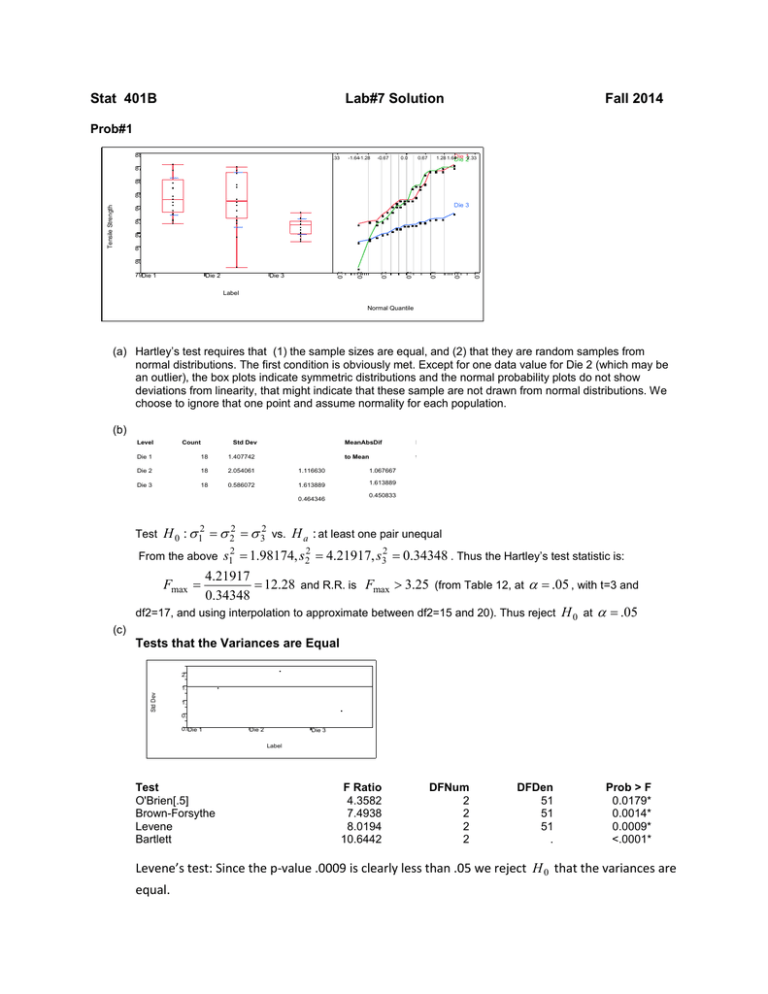
Stat 401B
Lab#7 Solution
Fall 2014
Prob#1
88
-1.64-1.28
.33
-0.67
0.67
0.0
Die
1.28 1.64
Die 1
22.33
87
86
Tensile Strength
85
Die 3
84
83
82
81
0.9
0.9
0.8
0.5
Die 3
0.2
Die 2
0.0
79Die 1
0.0
80
Label
Normal Quantile
(a) Hartley’s test requires that (1) the sample sizes are equal, and (2) that they are random samples from
normal distributions. The first condition is obviously met. Except for one data value for Die 2 (which may be
an outlier), the box plots indicate symmetric distributions and the normal probability plots do not show
deviations from linearity, that might indicate that these sample are not drawn from normal distributions. We
choose to ignore that one point and assume normality for each population.
(b)
Level
Std Dev
Count
MeanAbsDif
M
to Mean
t
Die 1
18
1.407742
Die 2
18
2.054061
1.116630
1.067667
Die 3
18
0.586072
1.613889
1.613889
0.464346
Test
0.450833
H 0 : σ 12 = σ 22 = σ 32 vs. H a : at least one pair unequal
= 1.98174, s22 = 4.21917, s32 = 0.34348 . Thus the Hartley’s test statistic is:
4.21917
Fmax =
= 12.28 and R.R. is Fmax > 3.25 (from Table 12, at α = .05 , with t=3 and
0.34348
df2=17, and using interpolation to approximate between df2=15 and 20). Thus reject H 0 at α = .05
2
From the above s1
(c)
Tests that the Variances are Equal
2.0
Std Dev
1.5
1.0
0.5
0.0Die 1
Die 2
Die 3
Label
Test
O'Brien[.5]
Brown-Forsythe
Levene
Bartlett
F Ratio
4.3582
7.4938
8.0194
10.6442
DFNum
2
2
2
2
DFDen
51
51
51
.
Prob > F
0.0179*
0.0014*
0.0009*
<.0001*
Levene’s test: Since the p-value .0009 is clearly less than .05 we reject H 0 that the variances are
equal.
Problem 2
(a) See JMP output.
(b)
564
16446
(
(c)
)
1785
536
12 54
(e) 2 72
5
51814
(
1456
2 72
(d)
164 13
)
4631
12 54
2 72
13 6
(f) See Excel table.
(g) See Excel table.
(h) See Excel table.
(
(i)
)
4631
(
)
3956
(
)
675
85
85% of the variability in gas consumption is explained by the linear regression model.
(j)
37 51
(k)
26
(l) 95
(2 16, 3 27)
,
(m)
1 46
,
Reject the null hypothesis at
of gas consumption.
5 There is sufficient evidence that temperature difference is a predictor
(n) Anova Table
Source
Regression
Error
Total
Df
1
18
19
Sum of Squares
3956
675
4631
1 5
,
Reject the null hypothesis at
5
Mean Square
3956
37
F
105
(o)
12 54
2 72
25
8 54
1
95
,
(p) 95
,
1
(
)
(
(77 17, 83 95)
)
(67 26, 93 87)
(q) See JMP output and additional table.
(r) The plot of residuals against predicted values suggests some concern for the assumption of homogeneity of
variance, since there is a megaphone shape pattern. The normal probability plot supports the assumption
of normality of errors, since the plotted points lie near a straight line.
(s)
:
8
:
8
(77 17, 83 95)
95
80 is contained in the interval so we fail to reject the null hypothesis. There is insufficient evidence that the
manufacturers contention is wrong.
JMP Output for Problem 2
Simple Linear Regression of Gas_KWh on Temp_Diff
Linear Fit
Gas_KWh = 12.642442 + 2.7168076*Temp_Diff
Summary of Fit
RSquare
RSquare Adj
Root Mean Square Error
Mean of Response
Observations (or Sum Wgts)
0.854202
0.846102
6.124408
89.27
20
Analysis of Variance
Source
Model
Error
C. Total
DF
1
18
19
Sum of Squares
3955.5713
675.1507
4630.7220
Mean Square
3955.57
37.51
F Ratio
105.4584
Prob > F
<.0001*
Parameter Estimates
Term
Intercept
Temp_Diff
Estimate
12.642442
2.7168076
Residual by Predicted Plot
Std Error
7.586442
0.264556
t Ratio
1.67
10.27
Prob>|t|
0.1129
<.0001*
Lower 95%
-3.296081
2.1609951
Upper 95%
28.580965
3.2726201
Actual by Predicted Plot
Residual by Row Plot
Residual Normal Quantile Plot
Excel Table for Problem 2
x
20.1
21.1
21.9
22.6
23.4
24.2
24.9
25.1
26
27.2
28.8
29.2
30.6
y
65.3
66.5
67.8
73.2
75.3
81.1
82.2
85.7
90.9
87.4
94.9
93.9
87.1
yhat
67.25027
69.96708
72.14053
74.04229
76.21574
78.38919
80.29095
80.83431
83.27944
86.53961
90.8865
91.97322
95.77675
30.8
32.6
32.4
34.8
35.9
36
36.5
84.2
106.6
111.3
100.9
101.9
110.1
119.1
96.32012
101.2104
100.667
107.1873
110.1758
110.4475
111.8059
ybar=
89.27
y-yhat
-1.95027476
-3.46708236
-4.34052844
-0.84229376
-0.91573984
2.71081408
1.90904876
4.86568724
7.6205604
0.86039128
4.01349912
1.92677608
-8.67675456
12.12011608
5.38963024
10.63299176
-6.28734648
-8.27583484
-0.3475156
7.2940806
SSTot=
SSE=
SSReg=
4630.722
675.1506631
3955.571351
SSReg+SSE=
4630.722014
y-ybar
-23.97
-22.77
-21.47
-16.07
-13.97
-8.17
-7.07
-3.57
1.63
-1.87
5.63
4.63
-2.17
yhatybar
-22.0197
-19.3029
-17.1295
-15.2277
-13.0543
-10.8808
-8.97905
-8.43569
-5.99056
-2.73039
1.616501
2.703224
6.506755
-5.07
17.33
22.03
11.63
12.63
20.83
29.83
7.050116
11.94037
11.39701
17.91735
20.90583
21.17752
22.53592
Additional Table for Problem 2
Temp_Diff
Gas_KWh
Predicted
Residual
20.1
21.1
21.9
22.6
23.4
24.2
24.9
25.1
26.0
27.2
28.8
29.2
30.6
30.8
32.6
32.4
34.8
35.9
36.0
36.5
25.0
65.3
66.5
67.8
73.2
75.3
81.1
82.2
85.7
90.9
87.4
94.9
93.9
87.1
84.2
106.6
111.3
100.9
101.9
110.1
119.1
.
67.25
69.97
72.14
74.04
76.22
78.39
80.29
80.83
83.28
86.54
90.89
91.97
95.78
96.32
101.21
100.67
107.19
110.18
110.45
111.81
80.56
-1.9503
-3.4671
-4.3405
-0.8423
-0.9157
2.7108
1.9090
4.8657
7.6206
0.8604
4.0135
1.9268
-8.6768
-12.120
5.3896
10.6330
-6.2873
-8.2758
-0.3475
7.2941
.
Lower 95%
Mean
61.91
65.08
67.61
69.80
72.29
74.75
76.88
77.48
80.15
83.61
87.99
89.04
92.61
93.10
97.44
96.96
102.5
105.0
105.2
106.4
77.18
Upper 95%
Mean
72.60
74.85
76.67
78.28
80.14
82.03
83.70
84.19
86.41
89.47
93.78
94.90
98.95
99.54
105.0
104.4
111.8
115.3
115.6
117.2
83.95
Lower 95%
Indiv
53.32
56.20
58.50
60.49
62.76
65.02
66.98
67.54
70.04
73.34
77.70
78.78
82.53
83.06
87.80
87.28
93.50
96.31
96.57
97.84
67.26
Upper 95%
Indiv
81.18
83.73
85.78
87.59
89.67
91.76
93.60
94.13
96.52
99.74
104.1
105.2
109.0
109.6
114.6
114.1
120.9
124.0
124.3
125.8
93.87