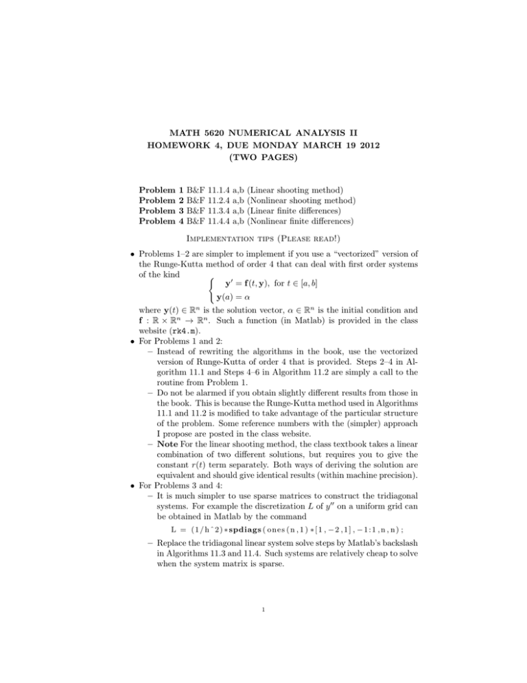
MATH 5620 NUMERICAL ANALYSIS II
HOMEWORK 4, DUE MONDAY MARCH 19 2012
(TWO PAGES)
Problem
Problem
Problem
Problem
1
2
3
4
B&F
B&F
B&F
B&F
11.1.4
11.2.4
11.3.4
11.4.4
a,b
a,b
a,b
a,b
(Linear shooting method)
(Nonlinear shooting method)
(Linear finite differences)
(Nonlinear finite differences)
Implementation tips (Please read!)
• Problems 1–2 are simpler to implement if you use a “vectorized” version of
the Runge-Kutta method of order 4 that can deal with first order systems
of the kind
(
y0 = f (t, y), for t ∈ [a, b]
y(a) = α
n
where y(t) ∈ R is the solution vector, α ∈ Rn is the initial condition and
f : R × Rn → Rn . Such a function (in Matlab) is provided in the class
website (rk4.m).
• For Problems 1 and 2:
– Instead of rewriting the algorithms in the book, use the vectorized
version of Runge-Kutta of order 4 that is provided. Steps 2–4 in Algorithm 11.1 and Steps 4–6 in Algorithm 11.2 are simply a call to the
routine from Problem 1.
– Do not be alarmed if you obtain slightly different results from those in
the book. This is because the Runge-Kutta method used in Algorithms
11.1 and 11.2 is modified to take advantage of the particular structure
of the problem. Some reference numbers with the (simpler) approach
I propose are posted in the class website.
– Note For the linear shooting method, the class textbook takes a linear
combination of two different solutions, but requires you to give the
constant r(t) term separately. Both ways of deriving the solution are
equivalent and should give identical results (within machine precision).
• For Problems 3 and 4:
– It is much simpler to use sparse matrices to construct the tridiagonal
systems. For example the discretization L of y 00 on a uniform grid can
be obtained in Matlab by the command
L = ( 1 / h ˆ 2 ) ∗ spdiags ( o n e s ( n , 1 ) ∗ [ 1 , − 2 , 1 ] , − 1 : 1 , n , n ) ;
– Replace the tridiagonal linear system solve steps by Matlab’s backslash
in Algorithms 11.3 and 11.4. Such systems are relatively cheap to solve
when the system matrix is sparse.
1
2
MATH 5620 NUMERICAL ANALYSIS II HOMEWORK 4, DUE MONDAY MARCH 19 2012 (TWO PAGES)
– The behavior of spdiags can be tricky if your sub/super diagonals
vary. This matlab code:
Q = [ 1 3 0
2 3 −1
3 3 −2
0 3 −3 ] ;
A = spdiags (Q, − 1 : 1 , 4 , 4 ) ;
constructs the matrix with entries:


3 −1
1 3 −2


A=

2
3 −3
3
3
So spdiags uses only the upper part of subdiagonals and the lower
part of superdiagonals.
– If you do not want to use spdiags you can create an n by n all zeros
sparse matrix with A=sparse(n,n); and then fill it entry by entry
(with a for loop).