Application 9.5 Heated Rod (p 628)
Diffusivity constant
O k:=0.15; k := 0.15
(1)
Length of the rod
O L := 50;
L := 50 (2)
Initial temperature
O u0 := 100; u0 := 100 (3)
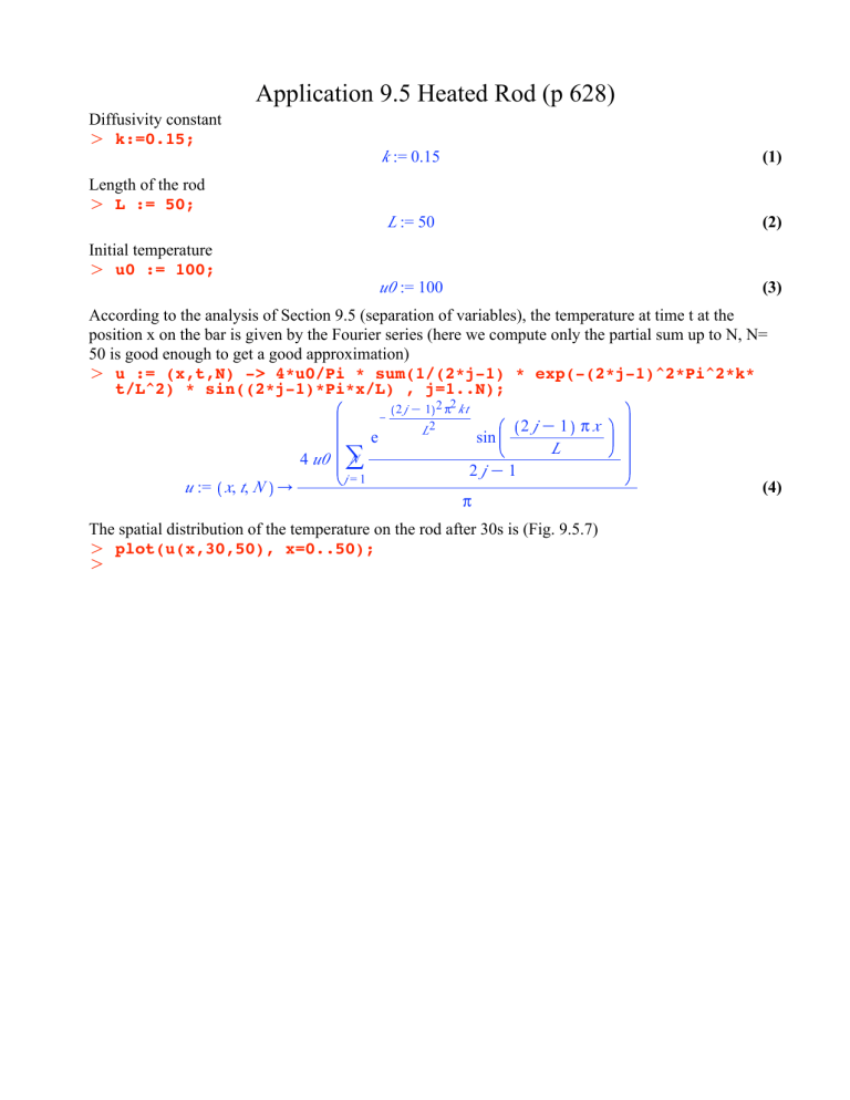
According to the analysis of Section 9.5 (separation of variables), the temperature at time t at the position x on the bar is given by the Fourier series (here we compute only the partial sum up to N, N=
50 is good enough to get a good approximation)
O u := (x,t,N) -> 4*u0/Pi * sum(1/(2*j-1) * exp(-(2*j-1)^2*Pi^2*k* t/L^2) * sin((2*j-1)*Pi*x/L) , j=1..N);
2 j K 1 2 p
2 k t u := x , t , N /
4 u0
> j = 1 e
K
L
2 p
sin
2 j K 1
2 j K
L
1 p x
(4)
The spatial distribution of the temperature on the rod after 30s is (Fig. 9.5.7)
O
O plot(u(x,30,50), x=0..50);

100
80
60
40
20
0
0 10 20 30 40 50 and after 30 min (Fig. 9.5.8). Because of symmetries the maximum temperature will be at the center of the interval (x=25)
O plot(u(x,30*60,50),x=0..50);

40
30
20
10
0
0 10 20 30 40 50
We can also see how the temperature at a particular point of the bar changes with time. Here is how the temperature at the midpoint evolves. The temperature over the rest of the bar is smaller (Fig. 9.5.9)
O plot({u(25,t,50),50}, t=0..7000);

100
90
80
70
60
50
40
30
20
10
0 1,000 2,000 3,000 4,000 5,000 6,000 7,000
Thus if we want to know how long it takes for the temperature on the rod to be less than 50C (so that we don't burn by holding it, for example), it is sufficient to look at the temperature on the midpoint because it is the hottest point of the rod. According to the previous plot it takes the system between
1000 and 2000 seconds for this to happen. Let us zoom in to find a better value:
O plot({u(25,t,50),50}, t=1000..2000);

70
60
50
40
1,000 1,200 1,400 1,600 1,800 2,000
From the plot the time would be between 1500 and 1600 seconds. We could continue zooming in
(narrowing the range of t around the intersection between the temperature curve and u=50), or we could also use the numerical methods built in Maple to find a numerical solution. Here we specify that the solution is in the range t=0..2000 (if you omit this argument to fsolve, Maple gets confused and gives you a negative time, which is non-physical! Of course, the range you specify here depends on the problem)
O T50 := fsolve(u(25,t,50) = 50 , t=0..2000);
T50 := 1578.115992
(5)
The time in minutes and seconds is then:
O printf("%d:%.2f\n",floor(T50/60), frac(T50/60)*60);
26:18.12
O