Math 3080 § 1.
Final Exam
Name:
Example
Treibergs
April 19, 2010
Problems mostly about material since 2nd midterm.
Problems taken from Prof. Roberts’ Math 3080 Exams given Spring 2004
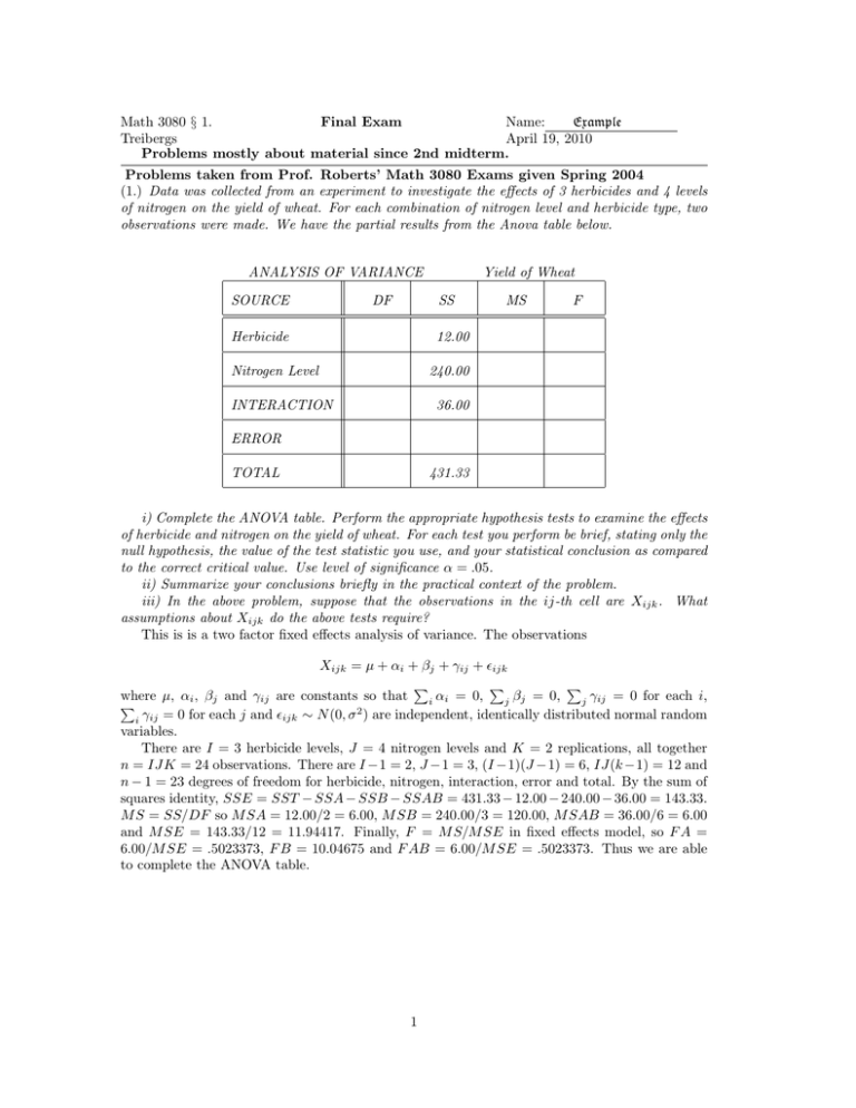
(1.) Data was collected from an experiment to investigate the effects of 3 herbicides and 4 levels
of nitrogen on the yield of wheat. For each combination of nitrogen level and herbicide type, two
observations were made. We have the partial results from the Anova table below.
ANALYSIS OF VARIANCE
SOURCE
DF
Yield of Wheat
SS
Herbicide
MS
F
12.00
Nitrogen Level
240.00
INTERACTION
36.00
ERROR
TOTAL
431.33
i) Complete the ANOVA table. Perform the appropriate hypothesis tests to examine the effects
of herbicide and nitrogen on the yield of wheat. For each test you perform be brief, stating only the
null hypothesis, the value of the test statistic you use, and your statistical conclusion as compared
to the correct critical value. Use level of significance α = .05.
ii) Summarize your conclusions briefly in the practical context of the problem.
iii) In the above problem, suppose that the observations in the ij-th cell are Xijk . What
assumptions about Xijk do the above tests require?
This is is a two factor fixed effects analysis of variance. The observations
Xijk = µ + αi + βj + γij + ijk
P
P
P
where µ, αi , βj and γij are constants so that i αi = 0,
j βj = 0,
j γij = 0 for each i,
P
2
γ
=
0
for
each
j
and
∼
N
(0,
σ
)
are
independent,
identically
distributed
normal random
ij
ijk
i
variables.
There are I = 3 herbicide levels, J = 4 nitrogen levels and K = 2 replications, all together
n = IJK = 24 observations. There are I −1 = 2, J −1 = 3, (I −1)(J −1) = 6, IJ(k −1) = 12 and
n − 1 = 23 degrees of freedom for herbicide, nitrogen, interaction, error and total. By the sum of
squares identity, SSE = SST − SSA − SSB − SSAB = 431.33 − 12.00 − 240.00 − 36.00 = 143.33.
M S = SS/DF so M SA = 12.00/2 = 6.00, M SB = 240.00/3 = 120.00, M SAB = 36.00/6 = 6.00
and M SE = 143.33/12 = 11.94417. Finally, F = M S/M SE in fixed effects model, so F A =
6.00/M SE = .5023373, F B = 10.04675 and F AB = 6.00/M SE = .5023373. Thus we are able
to complete the ANOVA table.
1
Source of Variation
DF
SS
MS
F
Herbicide
2
12.00
6.00
.5023373
Nitrogen
3
240.00
120.00
10.04675
Interaction
6
36.00
6.00
.5023373
Error
12
143.33
11.94
Total
23
431.33
The first test of hypothesis is whether interactions are significant
HAB
0
:
γij = 0
for all i, j;
HAB
1
:
γij 6= 0
for some i, j.
v.
Under HAB 0 , F AB ∼ f(I−1)(J−1),IJ(K−1) so we reject HAB 0 if F AB > f6,12 (.05) = 3.00. Since
F AB is less, we are unable to reject HAB 0 : the interactions are plausibly negligible.
The second test of hypothesis is whether the herbicide effect is significant
HA
0
:
αi = 0
for all i;
HA
1
:
αi 6= 0
for some i.
v.
Under HA 0 , F A ∼ fI−1,IJ(K−1) so we reject HA 0 if F A > f2,12 (.05) = 3.89. Since F A is less,
we are unable to reject HA 0 : the herbicide effect is plausibly negligible.
The final test of hypothesis is whether the nitrogen effect is significant
HB
0
:
βj = 0
for all j;
HB
1
:
βj 6= 0
for some j.
v.
Under HB 0 , F AB ∼ fJ−1,IJ(K−1) so we reject HAB 0 if F AB > f2,12 (.05) = 3.49. Since F B is
larger, we reject HAB 0 : the nitrogen effect is significant at the 0.05 level.
(2.) A study of the hours of relief provided by 5 different headache tablets was conducted on 25
patients assigned at random, 5 to each type of tablet. The mean and standard deviation of the
sample for each tablet is reported in the table below. Assume that the hours of relief for each
tablet was approximately normally distributed with the same variance for each tablet. Use this
information to answer the following questions.
A
B
C
D
E
Mean
5.44
7.90
4.30
2.98
6.96
Stdev
1.89
1.34
2.11
1.30
1.85
PP 2
The grand mean is X.. = 5.516 and
Xij = 929.974.
i) Set up the Anova table for this experiment. Do the sample results indicate that there is a
difference in the mean hours of relief offered by the different tablets? Use α = .05.
ii) Using Tukey’s method to determine which pairs of tablets differ significantly in the mean
hours of relief provided by the tablets. Use α = .05.
Let us construct the ANOVA table. This is a one-way fixed effects model. That means that
we assume the observations
Xij = µ + αi + ij
2
P
where µ, αi are constants so that i αi = 0 and ij ∼ N (0, σ 2 ) are independent, identically
distributed normal random variables. In this case there are I = 5 levels of the factor and J = 5
replicates and n = IJ = 25 observations. Hence the degrees of freedom
the tablet
P is2a I −1 = 4 for
A, I(J−1) = 20 for the error and IJ−1 = 24 for the total. SST = ij Xij
−n(Xcdot · )2 = 190.134.
P
SSA = J( i (X̄i· − X̄· · )2 ) = 78.4216. Thus SSE = SST − SSA = 169.3176 − 78.4216 = 90.896.
M S = SS/DF so M SA = 78.4216/4 = 19.6054 and M SE = 90.896/20 = 4.5448. Finally
F = M SA/M SE = 19.6054/4.5448 = 4.313809. The ANOVA table is
DF
SS
MS
F
A
4
78.4216
19.6054
4.313809
Error
20
90.896
4.5448
Total
24
169.3176
Source of Variation
To test the hypothesis whether the effect is significant
H0 :
αi = 0
for all i;
H1 :
αi 6= 0
for some i.
v.
Under H0 , F ∼ fI−1,I(J−1) so we reject H0 if F > f4,20 (.05) = 2.87. Since F is larger, we reject
H0 : the hours of relief are significantly different at the 0.05 level.
To determine which differences are significant, we compute the Tukey’s HSD. In this case the
critical value of the Studentized Range is q(.05, 5, 20) = 4.23 so
r
r
M SE
4.5448
HSD = q(α, I, I(J − 1))
= 4.23
= 4.03.
J
5
Only |X̄D − X̄B | > HSD and the other differences are smaller than HSD. Sorting the means,
we put Tukey Bars under subsets whose pairs that are not significantly different.
Mean
D
C
A
E
B
2.98
4.30
5.44
6.96
7.90
(3.) A random sample of 445 college students was classified according to frequency of marijuana
use and parental use of alcohol and psychoactive drugs. Does the data suggest that parental usage
and student usage are independent in the population sampled?
Student Usage
Parental Usage
Never
Occasional
Regular
Total
Neither
141
54
40
235
One
68
44
51
163
Both
17
11
19
47
Total
226
109
110
445
3
What is the null hypothesis here? Assuming the null hypothesis is true, what is the probability
and the expected number for the “Neither ∗ Never” cell? The total of the contributions to the test
statistic from all cells except “Neither ∗ Never” cell is: 18.5. Find the contribution from that cell
and state the value of this test statistic result. give the approximate p-value of your test statistic.
State what the p-value of your test statistic means in the practical terms of the problem. Finally,
what conclusion would you recommend and why?
This is a χ2 test for independence. The null hypothesis is
v.
H0 :
pij = pi· p·j
for all i, j;
H1 :
pij 6= pi· p·j
for some i, j.
Under H0 , the expected probability of parental neither and student never is p̂11 = p̂1· p̂·1 =
(235/445)(226/445) = 0.2681985. Thus the expected number is ê11 = p̂11 n = 445 × 0.2681985 =
119.3483. The test statistic is, according to the given data
X (yij − êij )2
(y11 − ê11 )2
=
+
χ =
êij
ê11
i,j
2
J
X
(i,j)6=(1,1)
(141 − 119.3483)2
(yij − êij )2
=
+ 18.5 = 22.4.
êij
119.3483
Under H0 , the statistic is distributed according to χ2(I−1)(J−1) . The P -value is thus P = P (χ24 >
22.4) < .005 from the table. (In fact, P = 0.0001689.) Thus we reject H0 : the data shows that
the rows and columns are not independent.
Problems taken from my Math 3080 Exams given Spring 2005
(1.)Complete the ANOVA table, given that there were five samples taken from each of the three
populations.
Source of
Variation
df
SS
MS
9.8
Treatment
Error
Total
31.6
4
f
P -value
F -crit
(2.)The yield of wheat in bushels per acre were compared for five different vaieties A, B, C, D,
E and at six different locations. Each variety was randomly assigned to a plot at each location.
The ANOVA table for the data, generated by Excel, is shown below, with α = .05. Use the table
to answer the questions.
Anova:
Two-Factor Without Replication
SUMMARY
A
B
C
D
E
Loc
Loc
Loc
Loc
Loc
Loc
1
2
3
4
5
6
Count
Sum
Average
6
6
6
6
6
206.2
193.7
217.8
220.7
187.2
34.36667
32.23333
36.3
36.73333
31.2
5
5
5
5
5
5
171.5
161.7
162.1
174.6
183.6
172.1
34.3
32.34
32.42
34.92
36.72
34.42
Variance
5.97467
2.23767
4.912
4.22167
3.816
8.285
7.163
5.152
11.972
5.897
6.717
ANOVA
Source of
Variation
Rows
Columns
Error
Total
SS
df
142.70467
67.77067
38.03933
248.51467
4
5
20
29
MS
35.67617
13.55413
1.90197
F
P-value
F crit
18.75751
7.12638
0.000001516
0.000565452
2.86608
2.71089
a. State the assumptions that are being made in order to do the ANOVA test.
Random blocks design which is the same as the two-factor without replication design.
P Xij =
µ
+
α
+
β
+
where
i
=
1,
.
.
.
,
I,
j
=
1,
.
.
.
,
J,
µ,
α
and
β
are
constants
so
that
i
j
ij
i
j
i αi = 0,
P
β
=
0,
∼
N
(0,
σ)
is
a
random
sample
taken
from
normal
RV.
j
ij
j
b. Do the data provide sufficient evidence to indicate (at the α = .05 level) a difference in
mean yield for the five varieties of wheat?
Yes. The P -value for fVariety is 0.00000152 < .05 so is significant.
c.If another plot at location 2 were planted variety C, what is your best guess of the yield?
Why?
Note x̄·· = 15 (34.37 + 32.23 + 36.30 + 36.73 + 31.20) = 34.4533. Since E(X32 ) = µ + α3 + β2 =
E(x̄3· ) + E(x̄·2 ) − E(x̄·· ) we take the estimator x̄3· + x̄·2 − x̄·· = 36.30 + 32.34 − 34.45 = 34.19.
(3.)From the data for problem (2), use Tukey’s procedure (at the α = 0.5 level) to identify significant differences among the different varieties. Order the means and indicate the relationship
between the means using underscoring.
q
Tukey’s test is to compare all differences simultaneously with w = q MJSE where the one
tailed, level α studentized range statistic for I = 5 levels is q = qα,I,(I−1)(J−1) = q.05,5,20 = 4.23.
q
So w = 4.23 · 1.90197
= 2.38.
6
Since x̄4,· − x̄1· = 2.36 < w < x̄4,· − x̄2· = 4.50, x̄1,· − x̄2· = 2.13 < w < x̄3,· − x̄2· = 4.07 and
x̄2,· − x̄5· = 1.03 < w < x̄1,· − x̄5· = 3.17, evidence allows us to find conclude that means E and
B do not differ; means B and A do not differ; means A, C and D do not differ; although C and
D differ from B, neither differs from A; although A and E differ from each other, neither differs
from B.
5
The underscoring pattern is:
E
B
A
C
D
31.20
32.23
34.37
36.30
36.73
==============
++++++++++++++
----------------------(3.)Consider the following experiment to test whether or not three different college entrance exams
are interchangeable. A list of all colleges in the United States with 100 or more students was
obtained, and 20 schools were randomly selected from the list. Then 30 students were randomly
sampled from each of the twenty schools and randomly divided into three groups of 10 students
each. The first group took Exam A, the second took Exam B, and the third took Exam C. Partial
results of the two way ANOVA with “Exam” as one of the factors and “School” as the other is
listed. State the model. What assumptions are made about the data in order to make the ANOVA
analysis? Complete the ANOVA table. Carry out the tests of the three hypotheses. What is your
conclusion?
Two factor mixed fixed/random effects model with replication. Xijk = µ + αi + Bj +PGij + εijk
for i = 1, . . . , I, j = 1, . . . J and k = 1, . . . , K where µ and αi are constant, such that i αi = 0.
2
2
, V (Gij ) = σG
The Bi , Gij and εijk are independent normal RV’s with mean zero and V (Bj ) = σB
2
and V (εijk ) = σ , constant, but unknown variances. A is the fixed effect (test) and B is the
random effect (School.) State the three hypotheses of interest, and their corresponding tests.
ANOVA
Source of
Variation
df
SS
Exam
2
School
19
Exam*School 38
Error
540
Total
599
589
2833
5738
46440
56650
MS
F
294.5
151.7
151.0
86.0
F crit
1.950
1.005
1.756
3.25
1.84
1.42
2
= 0. Compute fAB = MMSAB
HAB 0 : σG
SE to reject HAB 0 if fAB > f.05,38,540 . HA 0 : α1 =
SA
2
= 0. Compute
to reject HA 0 if fA > f.05,2,38 . HB 0 : σB
· · · = αI = 0. Compute fA = MMSAB
M SB
fB = M SAB to reject HB 0 if fB > f.05,19,38 .
The interaction term is significant. Normally this ends the analysis. It turns out that neither
other effect is significant.
(1.) Answer:
ANOVA
Source of
Variation
df
SS
MS
F
F crit
Treatment
Error
Total
2
12
14
19.6
12.0
31.6
9.8
1.0
9.8
3.89
6
(4.)In a study about ball bearing life, Box (1992) considered four fixed factors in the manufacturing
process: XX=type of ball, Y Y =cage design, ZZ=type of grease and W W =amount of grease and
lif e=relative time. Each of the factor had two levels: 1 =“standard” or 2 =“modified.” Test at
the 95% confidence level whether any of the main effects are significant. State your hypotheses.
Here is the printout of the data file. Also, here is a partial printout of the ANOVA table made
requesting all interactions of the four variables in the model. The rest of the entries in the table
were “undefined.”
XX YY ZZ WW
1 1 1 1
2 2 1 1
2 1 2 1
2 1 1 2
1 2 2 1
1 2 1 2
1 1 2 2
2 2 2 2
life
0.31
2.17
1.37
1.38
0.92
0.73
0.95
2.57
DF
1
1
1
1
1
1
1
1
CONSTANT
XX
YY
XX.YY
ZZ
XX.ZZ
YY.ZZ
XX.YY.ZZ
SS
13.52
2.622
0.70805
0.32
0.18605
0.0242
0.0002
0.09245
This is a 24 fixed effects experiment with half replication. From the eight data points and factor
levels, it is evident that XY ZW was the defining contrast and the experimental treatments were
the eight combinations with an even number of effects in common with XY ZW . In particular
XY Z is confounded with W . There is one degree of freedom for each of the sum of squares
in the table. To test whether any of the main effects are significant, we assume that there
are no interactions, and use the remaining sum of squares for a proxy for SSE. Thus we get
SSE1 = SSXY + SSXZ + SSY Z = 0.32 + 0.0242 + 0.0002 = 0.34440 and SST = SSX + SSY +
SSZ + SSW + SSE1 = 2.622 + 0.70805 + 0.18605 + 0.09245 + 0.34440 = 3.95295. The resulting
ANOVA table is thus
Source Var.
XX
YY
ZZ
WW
Error 1
Total
DF
1
1
1
1
3
7
Sum of Sq. Mean Square
2.622
2.622
0.70805
0.70805
0.18605
0.18605
0.09245
0.09245
0.34440
0.11480
3.95295
F
22.8397213
6.1676829
1.6206446
0.8053136
To test HA0 : α1 = 0 vs HA∞ : α∞ 6= 0 we accept HA1 if f > Fα,1,3 . The other factors are
tested similarly. For example, if α = 0.10 then F.10,1,3 = 5.54 so there is no strong evidence that
the ZZ and W W factors is nonzero whereas XX and Y Y are significantly nonzero. If α = .05
then F.05,1,3 = 10.13 so XX is significant at this level too.
7
More Problems
(1.) A 2001 study by Y. Li & J. Chen investigated the effect of levels of several factors on glucose
consumption (in g/L.) A single measurement is provided for each combination of factors.
A
-1
1
-1
1
-1
1
-1
1
B
-1
-1
1
1
-1
-1
1
1
C
-1
-1
-1
-1
1
1
1
1
Glucose Consumption
68.0
77.5
98.0
98.0
74.0
77.0
97.0
98.0
i) Compute estimates for the main effects and the interactions. Is it possible to compute an
error sum of squares? Explain.
Using Yates’s method (not in Rosenkrantz), where columns 1, 2, EC are sums in pairs followed
by differences in pairs of the previous columns, we get
Treatment Condition
xijk
1
2
Effects Contrast
Effect
SS = (contrast)2 /8
1
68
145.5
341.5
687.5
µ̂ = 85.94
59082.03
a
77.5
196
346
13.5
α̂1 = 1.69
22.78
b
98
151
9.5
94.5
β̂1 = 11.81
1116.28
ab
98
195
4
−11.5
AB
γ̂11
= −1.44
16.53
c
74
9.5
50.5
4.5
δ̂1 = 0.56
2.53
ac
77
0
44
−5.5
AC
γ̂11
= −.69
3.78
bc
97
3
−9.5
−6.5
BC
γ̂11
= −.81
2.64
abc
98
1
−2
7.5
ABC
γ̂111
= .94
7.03
Thus the effects are gotten by, e.g., α1 = (effects contrast)/8 = 13.5/8 = 1.69. It is not possible
to compute an error sum of squares, as there are no replications, there is no error sum of squares.
The alternative to Yates’ Method is to form the sums with the treatment basis signs. e1 =
(1, 1, 1, 1, 1, 1, 1, 1), ea = (−1, 1, −1, 1, −1, 1, −1, 1), eb = (−1, −1, 1, 1, −1, −1, 1, 1) and ec =
(−1, −1, −1, −1, 1, 1, 1, 1) so L1 = he1 , xijk i = 68 + 77.5 + · · · + 98 = 687.5, La = hea , xijk i =
−68 + 77.5 − 98 + 98 − · · · + 98 = 13.5, Lb = heb , xijk i = −68 − 77.5 + 98 + 98 − · · · + 98 = 94.5,
Lc = he1 , xijk i = −68 − · · · − 98 + 74 + · · · + 98 = 4.5. The others follow the same pattern. But
to get ANOVA table, these contrasts suffice.
ii) Are there any interactions among the larger effects? If so, which ones?
No, none of the interaction terms are nearly as large as the effect of factor B.
iii) Assume that it is known from past experience that the additive model holds. Add the sums
of squares for the interactions and use the result to in place of an error sum of squares to test the
hypothesis that the main effects are equal to zero.
8
If the additive model holds, then we may add the higher
P 2order interactions to 2get an estimate
for the σ 2 to replace the error sum of squares. We have
xijk = 60256.25 and x... /8 = 59082.03
so that SST = 60256.25 − 59082.03 = 1174.22. Thus SSE = SST − (SSA + SSB + SSC) =
1174.22 − (22.82 + 1116.28 + 2.53) = 32.63 so we construct the ANOVA table. There is strong
evidence that the main effect B is nonzero whereas not enough evidence to rule out that the other
effects are zero.
Source
df
Sum of Squares
Mean Square
f
P -value
A
1
22.78
22.78
2.78
.1699
B
1
116.28
1116.28
136.86
.00031
C
1
2.53
2.53
.31
.6072
Error
4
32.63
32.63
8.16
Total
7
1174.22
(2.) In a 25 experiment with half replication, suppose it is determined to confound E with ABCD.
Which treatment combinations should be used to carry out the experiment? List the resulting alias
pairs.
Since ABCD and E are complementary, the word ABCDE is being used to determine the
halves. Thus to list the set of experimental treatment combinations, we list all words which have
either an odd number of letters in common with the defining word ABCDE or an even number.
Thus, using the odd ones, the experimental treatments are
{A, B, C, D, E, ABC, ABD, ABE, ACD, ACE, ADE, BCD, BCE, BDE, CDE, ABCDE}
The aliased pairs are the words in the odd group and their generalized inteaction with the defining
word ABCDE, namely,
{1, ABCDE}
{A, BCDE}
{B, ACDE}
{C, ABDE}
{D, ABCE}
{E, ABCD}
{ABC, DE}
{ABD, CE}
{ABE, CD}
{ACD, BE}
{ACE, BD}
{ADE, AD}
{BCD, AE}
{BCE, AD}
{BDE, AC}
{CDE, AB}
9
(3.) A study “SN-Radio for the Quality Evaluation,” (Japanese Standards Association, 1988)
considered three mechanical and electrical factors that affect the measured sensitivity of a control
valve: A relative position of control bolt (center−0.5, center, cemter+0.5), B control bolt range
(2, 4, 5 and 7 mm) and C input voltage (100, 120, 150 V).
A1
B1
B2
B3
C1
151 135
178 171
204 190
C2
151 135
180 173
205 190
C3
151 138
181 174
206 192
A2
B1
B2
B3
156
183
210
148
168
204
158
183
211
149
170
203
158
183
213
150
172
204
A3
B1
B2
B3
161
189
215
145
182
202
162
191
216
148
184
203
163
192
217
148
183
205
Perform an analysis of variance to test for significant main and interaction effects. Find the
coefficient of determination, R2 . State the model, the test statistics, the rejection regions, and
your conclusions. The partial R output, interaction plots and diagnostic plots are attached.
Comment about what each plot says about the appropriateness of the model.
\Response: sensitivity
Df Sum Sq Mean Sq F value
Pr(>F)
A
2 1133.6
566.8
8.2991 0.001551
B
2 26896.3 13448.1 196.9086 < 2.2e-16
C
2
40.1
20.1
0.2939 0.747686
A:B
4
216.5
54.1
0.7926 0.540317
A:C
4
1.6
0.4
0.0060 0.999924
B:C
4
2.3
0.6
0.0084 0.999850
A:B:C
8
2.6
0.3
0.0047 1.000000
Residuals 27 1844.0
68.3
10
This is a three-way fixed effects anova with replicates. The model is
yijk` = µ + αi + βj + γk + (αβ)ij + (αγ)ik + (βγ)jk + (αβγ)ijk + ijk`
P
P
where
µ, αi , P
βj , γk , (αβ)ij , (αγ)ik , (βγ)
= 0, j βj = 0,
P
P jk , (αβγ)ijk are constants
P such that i αiP
all k, k (αγ)ik for all
k γk = 0,
i (αβ)ij =
P
P0 for all j, j (αβ)
Pij = 0 for all i, i (αγ)ik for P
i, j (βγ)jk for all k, k (βγ)jk for all j, i (αβγ)ijk = 0 for all (j, k), j (αβγ)ijk = 0 for all
P
(i, k), k (αβγ)ijk = 0 for all (i, j) and ijk` ∼ N (0, σ 2 ) are IID normal variables. In our case,
I = J = K = 3, L = 2.
The first test of hypothesis is whether three-way interactions are significant
HABC
0
:
(αβγ)ijk = 0
for all i, j, k;
HABC
1
:
(αβγ)ijk 6= 0
for some i, j, k.
v.
Under HABC 0 , F ABC ∼ f(I−1)(J−1)(K−1),IJK(L−1) so we reject HABC 0 if F ABC > f8,27 (.05).
Since the P value is P = 1.000, we are unable to reject HABC 0 : the 3-way interactions are
plausibly negligible.
The second tests of hypothesis is whether two-way interactions are significant. BC and AC
are similar to AB
HAB
0
:
(αβ)ij = 0
for all i, j;
HAB
1
:
(αβ)ij 6= 0
for some i, j.
v.
Under HAB 0 , F AB ∼ f(I−1)(J−1),IJK(L−1) so we reject HAB 0 if F AB > f4,27 (.05). Since the
P value is P = .540, we are unable to reject HAB 0 . Similarly, the P -values for HAC0 and HBC0
are both .999, we fail to reject those also: all 2-way interactions are plausibly negligible.
11
The last tests of hypothesis is whether the main effects are significant. The B and C effects
are tested similarly.
HA
HA
0
:
αi = 0
for all i;
1
:
αi 6= 0
for some i.
v.
Under HA 0 , F A ∼ fI−1,IJK(L−1) so we reject HA 0 if F A > f2,27 (.05). Since the P value is
P = .0016, we reject HA 0 . Similarly, the P -values for HB0 is P = 2.2 × 10−16 so we reject HB0
also. The P value for HC0 is .748, we fail to reject it: the main A and B effects are significant,
the C effect is not. We could perform Tukey’s HSD family comparisons on the A and B factors
at this point.
The design plot shows that factor B seems to have a large influence on the sensitivity. The
interaction plot shows that the lines are quite parallel, so we expect no AB interaction.
The box plot shows that the B factor accounts for widely different means. The size of the
boxes are similar, indicating the same variance for each level of the factor B are approximately
equal as we require of the model.
The plot of standardized residuals v. fitted values again shows that the data is “tubular,”
meaning that the spread is constant for different fitted values, as required of the model. This data
has a curious almost perfect symmetry suggesting that the B factor has symmetric influence.
The plot of fitted values ŷijk` versus observed values yijk` shows good alignment with the 45◦
line, again showing that the variance is uniform across the data, as we expect. The spread is not
large indicating that the model explains a lot of the variation.
Finally, the QQ-plot is significantly S-shaped. In other words, the large observed values of the
residuals are not as large as the corresponding normal quantiles: the distribution of the residuals
light tailed and is not very normal. In this case, a transformation of the data is in order. In fact
the transformation z = ((y − µ̂)/s)3 spreads the points and straightens our the S-shape.
To compute the coefficient of determination, SST = SSA + SSB + · · · + SSABC = 1133.6 +
26896.3 + 40.1 + 216.5 + 1.6 + 2.3 + 2.6 + 1844.0 = 30137.0 so
R2 = 1 −
1844.0
SSE
=1−
= .9388.
SST
30137.0
(4.) Consider a balanced one-way random effects analysis of variance model.
a. State the model and its assumptions.
b. Prove the sum of squares identity SST = SSA + SSE.
c. Find E(SSA) and E(SSE) for this model.
a. The balanced single factor random-effects model assumes that the observations are random
variables with I factors and the same number J observations per level
Yij = µ + Ai + ij
for all i = 1, . . . , I and j = 1, . . . , J where µ is constant, and the Ai ’s and ij ’s are mutually
2
independent random variables such that Ai ∼ N (0, σA
) for each i and ij ∼ N (0, σ 2 ) for each i, j
are normal, where σA and σ are two constants.
b. Using the usual dot notation to indicate summing over a subscript or bar-dot for averaging,
12
we have to relate three sums of squares
SST =
I X
J
X
Yij − Ȳ··
2
=
i=1 j=1
SSA =
I X
J
X
i=1 j=1
I X
J
X
Ȳi· − Ȳ··
2
=J
i=1 j=1
SSE =
I X
J
X
Yij2 − IJ Ȳ··2 ,
I
X
Yi·2 − IJ Ȳ··2 ,
i=1
Yij − Ȳi·
2
=
i=1 j=1
I X
J
X
Yij2 − J
i=1 j=1
I
X
Ȳi·2 .
i=1
The vanishing of the cross term happens for any model because
I X
J
X
Yij − Ȳi·
I
J
I
X
X
X
Ȳi· − Ȳ·· =
Ȳi· − Ȳ··
Yij − Ȳi· =
Ȳi· − Ȳ·· J Ȳi· − J Ȳi· = 0.
i=1 j=1
i=1
j=1
i=1
Hence
SST =
J
I X
X
Yij − Ȳ··
2
i=1 j=1
=
J
I X
X
Yij − Ȳi· + Ȳi· − Ȳ··
2
i=1 j=1
=
J n
I X
X
Yij − Ȳi·
2
+ 2 Yij − Ȳi·
2 o
Ȳi· − Ȳ·· + Ȳi· − Ȳ··
i=1 j=1
= SSE + 0 + SSA.
c. The expected values of the sum of squares uses the formula for variance of a random
variable X, namely V(X) = E(X 2 ) − E2 (X). Thus, using independence,
E(Yij ) = E (µ + Ai + ij ) = µ,
E(Yij2 )
2
= V(Yij ) + E2 (Yij ) = V (µ + Ai + ij ) + µ2 = σA
+ σ 2 + µ2 ,
J
J
J
1X
1X
1X
Yij =
(µ + Ai + ij ) = µ + Ai +
ij
J j=1
J j=1
J j=1


J
X
1
ij  = µ,
E(Ȳi· ) = E µ + Ai +
J j=1


J
X
1
1
2
E(Ȳi·2 ) = V µ + Ai +
ij  + E2 (Ȳi· ) = σA
+ σ 2 + µ2 ,
J j=1
J


I
I
J
I
I
J
1X
1 X
1X 
1X
1 XX
Ȳ·· =
Ȳi· =
µ + Ai +
ij = µ +
Ai +
ij
I i=1
I i=1
J j=1
I i=1
IJ i=1 j=1


I
I X
J
X
X
1
1
Ai +
ij  = µ
E(Ȳ·· ) = E µ +
I i=1
IJ i=1 j=1


I
I X
J
X
X
1
1
1 2
1 2
E(Ȳ··2 ) = V(Ȳ·· ) + E2 (Ȳ·· ) = V µ +
Ai +
ij  + µ2 = σA
+
σ + µ2
I i=1
IJ i=1 j=1
I
IJ
Ȳi· =
13
Putting these together we have the formulæ for the expectations of the sums of squares
!
I
I
X
X
2
2
E(SSA) = E J
Ȳi· − IJ Ȳ·· = J
E Ȳi·2 − IJ E Ȳ··2
i=1
=J
I X
i=1
2
σA
i=1
1
+ σ 2 + µ2
J
− IJ
1 2
1 2
σ +
σ + µ2
I A IJ
2
= J(I − 1)σA
+ (I − 1)σ 2
and


I X
J
I
X
X
E(SSE) = E 
Yij2 − J
Ȳi·2 
i=1 j=1
=
I X
J
X
i=1
I
X
E Ȳij2 − J
E Ȳi·2
i=1 j=1
=
I X
J
X
i=1
2
σA
2
2
+σ +µ
−J
i=1 j=1
I X
i=1
2
σA
1
+ σ 2 + µ2
J
= I(J − 1)σ 2 .
These agree with equations (12.22 − 12.23) of text (WAY TO GO UTES!)
(5.) Consider a 23 fixed effects analysis of variance model with n replicates per cell. Show that
SSAB = L2ab /(8n), where Lab is the contrast corresponding to the experimental condition ab.
The contrast basis vectors are e1 = (1, 1, 1, 1, 1, 1, 1, 1), ea = (−1, 1, −1, 1, −1, 1, −1, 1), eb =
(−1, −1, 1, 1, −1, −1, 1, 1) so their componentwise product is eab = (1, −1, −1, 1, 1, −1, −1, 1).
The cell sums are denoted (1), (a) (b), (ab) and so on. Let the vector of cell sums be V =
((1), (a), (b), (ab), (c), (ac), (bc), (abc)). Then the contrast is the inner product
Lab = heab , V i = (1) − (a) − (b) + (ab) + (c) − (ac) − (bc) + (abc).
On the other hand, in the model
yijk` = µ + αi + βj + γk + (αβ)ij + (αγ)ik + (βγ)jk + (αβγ)ijk + ijk`
the side conditions (see problem 3.) imply
(αβ)00 + (αβ)01 = (αβ)01 + (αβ)11 = (αβ)10 + (αβ)11 = 0
so
(αβ)11 = −(αβ)01 = −(αβ)10 = (αβ)00 .
\ij satisfy the same equations. Hence their squares are all equal and
The estimators (αβ)
SSAB =
2 X
2 X
2 X
n
X
i=1 j=1 k=1 `=1
14
2
2
[ = 8n(αβ)
\
(αβ)
11 .
ij
But the estimator for the effect is given by
\
(αβ)
11 = Ȳ11·· − Ȳ1··· − Ȳ·1·· + Ȳ····
4Y11·· − 2Y1··· − 2Y·1·· + Y····
=
8n
4Y110· + 4Y111· − 2Y100· − 2Y110· − 2Y101· − 2Y111· − 2Y010· − 2Y110· − 2Y011· − 2Y111·
=
8n
Y000· + Y100· + Y010· + Y110· + Y001· + Y101· + Y011· + Y111·
+
8n
Y000· − Y100· − Y010· + Y110· + Y001· − Y101· − Y011· + Y111·
=
8n
(1) − (a) − (b) + (ab) + (c) − (ac) − (bc) + (abc)
Lab
=
=
.
8n
8n
Hence we complete the computation
2
\
SSAB = 8n(αβ)
11 = 8n
Lab
8n
2
=
L2ab
.
8n
(5.) Consider a 23 fixed effects analysis of variance model with n replicates per cell. Show that
the sum of squares identity holds SST = SSE + SSA + SSB + SSAB + SSC + SSAC + SSBC +
SSABC.
P P P P 2
2
follows just like in problem 4a. Using
The fact that SST −SSE = i j k ` Ȳijk·
−8nȲ····
2
the fact that SSf actor = Lf actor /(8n) for all factors, the result follows from a basic fact of linear
algebra. Observe that all basis vectors e1 = (1, 1, 1, 1, 1, 1, 1, 1), ea = (−1, 1, −1, 1, −1, 1, −1,√
1),
eb = (−1, −1, 1, 1, −1, −1, 1, 1), eab = (1, −1,
−1,
1,
1,
−1,
−1,
1)
and
so
on.
All
have
length
8
√
√
and are orthogonal. Thus the vectors e1 / 8, ea / 8, . . . are orthonormal. Thus the orthogonal
decomposition of the vector V = ((1), (a), (b), (ab), (c), (ac), (bc), (abc)) into the orthonormal basis
is
e1
ea
eabc
V = c1 √ + ca √ + · · · cabc √
8
8
8
where cf actor is gotten by orthogonal projection
ef actor
L actor
√ i = f√
.
8
8
√
It follows that the square length of the vector V / n in R8 is
cf actor = hV,
1 X
1 X
1 X
n
X
i=0 j=0 k=0 `=1
2
Ȳijk·
=
|V |2
c2 + c2a + · · · + c2abc
= 1
n
n
=
L21 + L2a + · · · L2abc
2
= 8nȲ····
+ SSA + · · · + SSABC,
8n
2
since SSf actor = L2f actor /(8n) and Y···· = L1 . Subtracting 8nȲ····
completes the computation.
15