Math 3080 § 1.
Treibergs
First Midterm Exam
Name:
Solutions
February 10, 2010
1. The article “Flexible Pavement Evaluation. . . ” (Transportation Eng. J., 1977) used simple
regression to study the relationship between pavement deflection and surface temperature
at various locations on a state highway. Let x be temperature (F ◦ ) and y be the deflection
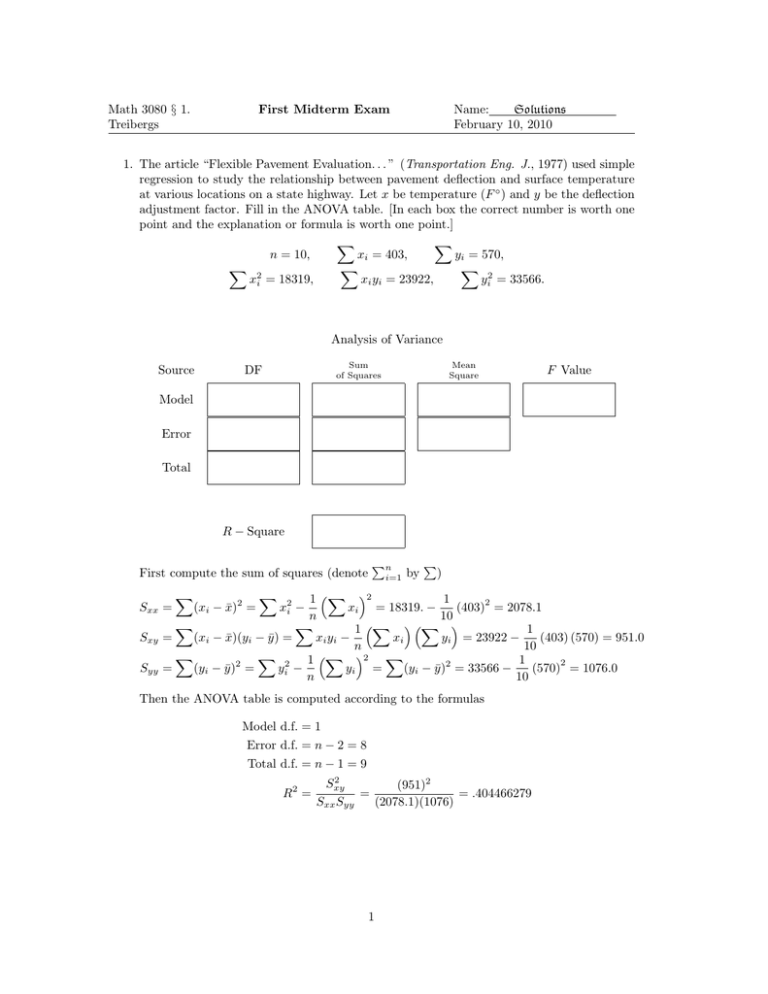
adjustment factor. Fill in the ANOVA table. [In each box the correct number is worth one
point and the explanation or formula is worth one point.]
X
X
n = 10,
xi = 403,
yi = 570,
X
X
X
x2i = 18319,
xi yi = 23922,
yi2 = 33566.
Analysis of Variance
Source
Sum
of Squares
DF
Mean
Square
F Value
Model
Error
Total
R − Square
First compute the sum of squares (denote
Syy
i=1
by
P
)
1
1 X 2
2
xi = 18319. −
(403) = 2078.1
x2i −
n
10
X
X
1 X X 1
=
(xi − x̄)(yi − ȳ) =
xi yi −
xi
yi = 23922 −
(403) (570) = 951.0
n
10
X
X
1
1 X 2 X
2
yi =
(yi − ȳ)2 = 33566 −
(570) = 1076.0
=
(yi − ȳ)2 =
yi2 −
n
10
Sxx =
Sxy
Pn
X
(xi − x̄)2 =
X
Then the ANOVA table is computed according to the formulas
Model d.f. = 1
Error d.f. = n − 2 = 8
Total d.f. = n − 1 = 9
R2 =
2
Sxy
(951)2
=
= .404466279
Sxx Syy
(2078.1)(1076)
1
SST = Syy = 1076
2
Sxy
(951)2
(= R2 · SST ) =
= 435.2057168
Sxx
2078.1
SSE = SST − SSR = 1076.0 − 435.2 = 640.7942832
SSR
435.2057168
M SR =
=
= 435.2057168
Model d.f.
1
SSE
640.7942832
M SE =
=
= 80.0992855
Error d.f.
8
M SR
435.2057168
F =
=
= 5.433328326.
M SE
80.0992855
SSR =
The ANOVA table consists of
Analysis of Variance
Source
DF
Sum
of Squares
Mean
Square
F Value
Model
Model d.f.
SSR
M SR
F
Error
Error d.f.
SSE
M SE
Total
Total d.f.
SST
R − Square
R2
Filling in the values
Analysis of Variance
Source
DF
Sum
of Squares
Mean
Square
F Value
Model
1
435.2
435.2
5.4333
Error
8
640.8
80.10
Total
9
1076.0
R − Square .4045
2
2. The study “Susceptability of Mice to Audiogenic Seizure. . . ” (Science, 1976) reports on
different injection treatments on the frequencies of seizures. What is the expected count of
mice in the study that were treated with Sham that exhibited Wild Running? Does the data
suggest that the true percentages in the different response categories depend on the nature
of the injection treatment? State and test the appropriate hypothesis at the α = .005 level
using the (partial) SAS output.
The FREQ Procedure:
Table of treatment by response
treatment
response
Frequency
Percent
Row Pct
Col Pct
|
|
|
|No
|Wild
|Clonic |Tonic
| Total
|Response|Running |Seizure |Seizure |
---------------+--------+--------+--------+--------+
Theinylalanine |
21 |
7 |
24 |
44 |
96
|
4.96 |
1.65 |
5.67 | 10.40 | 22.70
| 21.88 |
7.29 | 25.00 | 45.83 |
| 19.81 | 15.91 | 25.26 | 24.72 |
---------------+--------+--------+--------+--------+
Solvent
|
15 |
14 |
20 |
54 |
103
|
3.55 |
3.31 |
4.73 | 12.77 | 24.35
| 14.56 | 13.59 | 19.42 | 52.43 |
| 14.15 | 31.82 | 21.05 | 30.34 |
---------------+--------+--------+--------+--------+
Sham
|
23 |
10 |
23 |
48 |
104
|
5.44 |
2.36 |
5.44 | 11.35 | 24.59
| 22.12 |
9.62 | 22.12 | 46.15 |
| 21.70 | 22.73 | 24.21 | 26.97 |
---------------+--------+--------+--------+--------+
Unhandled
|
47 |
13 |
28 |
32 |
120
| 11.11 |
3.07 |
6.62 |
7.57 | 28.37
| 39.17 | 10.83 | 23.33 | 26.67 |
| 44.34 | 29.55 | 29.47 | 17.98 |
---------------+--------+--------+--------+--------+
Total
106
44
95
178
423
25.06
10.40
22.46
42.08
100.00
Statistics for Table of treatment by response
Statistic
DF
Value
Prob
-----------------------------------------------------Chi-Square
9
27.6642
0.0011
Sample Size = 423
The expected count in the (Sham, Wild Running) cell is
e3,2 = n3,• · p̂2 = n3,• ·
3
n•,2
104 · 44
=
= 10.818.
n•,•
423
This is a χ2 -test of homogeneity. Let pij denote the probability that the a mouse receiving
the i-th treatment will exhibit the jth response. The null hypothesis is that the response
does not depend on the treatment, or,
H0 :p1j = p2j = p3j = p4j = pj for all j = 1, 2, 3, 4.
H1 :H0 is false: pij 6= pi0 j for some i, i0 , j ∈ {1, 2, 3, 4} where i 6= i0 .
The output computes the statistic
4 X
4
X
(nij − eij )2
= 27.6642.
χ =
eij
i=1 j=1
2
Since all expected cell sizes eij ≥ 5 (since SAS did not give an expected count below 5
warning), the statistic has approximately the χ2 distribution with (r − 1)(c − 1) = 3 · 3 = 9
degrees of freedom. According to the output, the P -value is .0011 < α = .005 so we reject
the null hypothesis: there is strong evidence that the response depends on the treatment.
4
3. The study of the sterility of a fruit fly “Hybrid Dysgenesis. . . ” (Genetics, 1979) proposed
that the number of ovaries that develop is a binomial random variable with density
2 x
p(x) =
p (1 − p)2−x ,
for x = 0, 1, 2
x
for some 0 < p < 1. Test whether the data is consistent with this model.
n1 + 2n2
[Hint: the MLE turns out to be p̂ =
which is p̂ = .0843 for these numbers.]
2(n0 + n1 + n2 )
x = No. Ovaries Developed:
nx = Observed Count:
0
1
2
1212
118
58
We use a χ2 -goodness of fit test where the cell probabilities are not completely specified.
Using the M LE for p gives the estimate of cell probabilities and cell frequencies ex = p(x)n
where p̂ is used to compute p(x). Thus
x = No. Ovaries Developed:
0
1
2
Total
nx = Observed Count:
1212
118
58
1388
p(x) = Model Cell Prob.
(1 − p)2
2p(1 − p)
p2
1
Estimated p(x) (not needed)
.83850649
.15438702
.00710649
1
ex = np(x) = Expected Cell Count
1163.847008
214.289184
9.863808
1388
1.992281
43.266798
234.908561
280.1676
2
(nx − ex )
ex
Since we estimated k = 1 parameter, the χ2 statistic has approximately a χ2 distribution
with c − 1 − k = 3 − 1 − 1 = 1 degree of freedom for large n. Since the expected cell counts
exceed 5, by our rule of thumb, the test is applicabile.
The null hypothesis is
H0 : P ( x ovaries develop) = p(x) for x = 0, 1, 2 and for some parameter 0 < p < 1
Using the MLE for p gives the χ2 statistic
χ2 =
2
X
(nx − ex )2
ex
x=0
= 280.2.
The critical value for one degree of freedom χ21 (.005) = 7.879. Since our statistic is greater,
we reject the null hypothesis: the data indicates stongly that the binomial distibution does
not provide a good model.
5
4. Consider the simple regression model for i = 1, . . . , n
Yi = β0 + β1 xi + i
where i ∼ N (0, σ 2 ) are IID normal random variables. Let Ŷi = β̂0 + β̂1 xi be the predicted
value. Show that
n
X
xi (Yi − Ŷi ) = 0.
i=1
Using the formula β̂0 = ȳ − β̂1 x̄, the predicted values can be rewritten
Ŷi = β̂0 + β̂1 xi = Ȳ − β̂1 x̄ + β1 xi = ȳ + β̂1 (xi − x̄).
Thus
n
X
n n
o
X
xi (Yi − Ŷi ) =
xi (Yi − Ȳ ) − xi β̂1 (xi − x̄)
i=1
i=1
n n
o
X
=
xi (Yi − Ȳ ) − x̄(Yi − Ȳ ) − xi β̂1 (xi − x̄) + x̄β̂1 (xi − x̄)
i=1
=
n
X
(xi − x̄)(Yi − Ȳ ) − β̂1
i=1
n
X
(xi − x̄)2
i=1
Sxy
· Sxx
= Sxy −
Sxx
= 0.
We have used the formula β̂1 =
Problem 1, and the fact that
n
X
Sxy
where Sxx and Sxy are defined as in the solution to
Sxx
Yi − Ȳ =
!
Yi
n
−n·
i=1
i=1
and similarly
n
X
1X
Yi
n i=1
!
P
(xi − x̄) = 0 so that
n
X
n
X
x̄ Yi − Ȳ = 0 =
x̄β̂1 (xi − x̄) .
i=1
i=1
6
=0
5. A study of the strength of titanium welds by Harwig et. al., (Welding Journal, 2001),
compared the oxygen content in parts per thousand (xi ) to strength in ksi (yi ). The model
is yi = β0 + β1 xi + i where i are IID N (0, σ 2 ) variables. What is the estimate for the
expected strength if the oxygen content is 1.70 parts per thousand? Find an α = .05 lower
one sided confidence interval for β1 . Does the data strongly indicate that β1 > 10.00?
Formulate the null and alternative hypotheses. Test at the α = 0.05 level.
R version 2.7.2 (2008-08-25)
Copyright (C) 2008 The R Foundation for Statistical Computing
> mean(OxygenContent); mean(Strength)
[1] 1.519655
[1] 75.49655
> fit <- lm(Strength ~ OxygenContent); summary(fit); anova(fit)
Call:
lm(formula = Strength ~ OxygenContent)
Residuals:
Min
1Q
Median
3Q
Max
-10.0185 -3.6639 -0.1139
4.4977 12.6515
Coefficients:
Estimate Std. Error t value Pr(>|t|)
(Intercept)
49.780
7.751
6.423
7e-07 ***
OxygenContent
16.923
5.050
3.351 0.00239 **
--Signif. codes: 0 *** 0.001 ** 0.01 * 0.05 . 0.1
1
Residual standard error: 5.841 on 27 degrees of freedom
Multiple R-squared: 0.2937,Adjusted R-squared: 0.2676
F-statistic: 11.23 on 1 and 27 DF, p-value: 0.002391
Analysis of Variance Table
Response: Strength
Df Sum Sq Mean Sq F value
Pr(>F)
OxygenContent 1 383.09 383.09 11.229 0.002391 **
Residuals
27 921.14
34.12
--Signif. codes: 0 *** 0.001 ** 0.01 * 0.05 . 0.1
1
The estimate of expected strength when x∗ = 1.70 is done by evaluating the regression line
at the point
∗ ) = β̂ + β̂ x∗ = 49.780 + 16.923 · 1.70 = 78.5.
\
E(Y
0
1
β̂1 is normally distributed so the standardization using it’s standard error is t-distributed
with n − 2 degrees of freedom. Here n = 29. Thus with α = .05 confidence, E(β̂1 ) = β1 lies
in the lower one-sided confidence interval (from the output)
β̂1 − s(β̂1 )tn−2 (α), ∞ = 16.923 − (5.050)(1.703), ∞ = 8.322, ∞ .
The proposed null and alternative hypotheses are
H0 :β1 = 10.00;
H1 :β1 > 10.00.
10.00 lies in the confidence interval above, so that with α = .05 confidence we accept the
null hypothesis: this study does not provide strong evidence that β1 > 10.00.
7