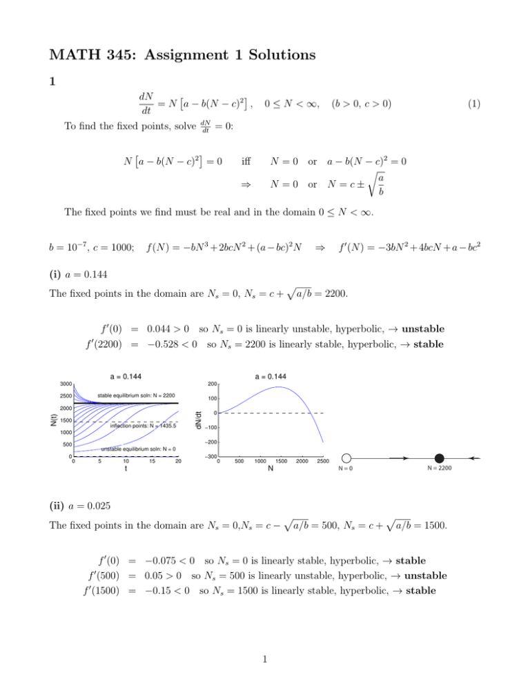
MATH 345: Assignment 1 Solutions
1
dN
= N a − b(N − c)2 ,
dt
To find the fixed points, solve dN
= 0:
dt
N a − b(N − c)2 = 0
0 ≤ N < ∞,
(b > 0, c > 0)
(1)
N = 0 or a − b(N − c)2 = 0
r
a
N = 0 or N = c ±
b
iff
⇒
The fixed points we find must be real and in the domain 0 ≤ N < ∞.
b = 10−7 , c = 1000;
f (N ) = −bN 3 + 2bcN 2 + (a − bc)2 N
⇒
f 0 (N ) = −3bN 2 + 4bcN + a − bc2
(i) a = 0.144
The fixed points in the domain are Ns = 0, Ns = c +
p
a/b = 2200.
f 0 (0) = 0.044 > 0 so Ns = 0 is linearly unstable, hyperbolic, → unstable
f 0 (2200) = −0.528 < 0 so Ns = 2200 is linearly stable, hyperbolic, → stable
a = 0.144
a = 0.144
3000
200
stable equilibrium soln: N = 2200
2500
100
1500
inflection points: N = 1435.5
dN/dt
N(t)
2000
0
−100
1000
−200
500
0
unstable equilibrium soln: N = 0
−300
0
5
10
15
20
0
500
1000
t
1500
N
2000
2500
N=0
N = 2200
(ii) a = 0.025
The fixed points in the domain are Ns = 0,Ns = c −
p
p
a/b = 500, Ns = c + a/b = 1500.
f 0 (0) = −0.075 < 0 so Ns = 0 is linearly stable, hyperbolic, → stable
f 0 (500) = 0.05 > 0 so Ns = 500 is linearly unstable, hyperbolic, → unstable
f 0 (1500) = −0.15 < 0 so Ns = 1500 is linearly stable, hyperbolic, → stable
1
a = 0.025
a = 0.025
3000
30
2500
20
stable equilibrium soln: N = 1500
dN/dt
N(t)
2000
1500
1000
0
unstable equilibrium soln: N = 500
−10
500
0
10
stable equilibrium soln: N = 0
−20
0
5
10
15
20
0
500
t
1000
1500
N
N=0
N = 500
(iii) a = −0.015
The only fixed point in the domain is Ns = 0.
f 0 (0) = −0.115 < 0 so Ns = 0 is linearly stable, hyperbolic, → stable
a = −0.015
a = −0.015
3000
5
2500
0
stable equilibrium soln: N = 0
−5
dN/dt
N(t)
2000
1500
−10
1000
−15
500
−20
0
−25
0
5
10
t
15
20
0
200
400
600
N
2
800
1000
1200
N=0
N = 1500
2
a = 0.025
3000
2500
2500
2000
2000
N(t)
N(t)
a = 0.144
3000
1500
1000
1000
500
500
0
0
10
20
30
40
0
50
t
a = −0.015
2500
2000
1500
1000
500
0
0
10
20
30
0
10
20
30
t
3000
N(t)
1500
40
50
t
3
40
50
3: Dimensionless form
For (1) to make sense, a should have units of yr−1 , b should have units yr−1 individuals−2 , c should
have units individuals.
, τ = Bt where A has units of individuals, B has units of yr, with values chosen
Let x = N
A
below. Substituting into (1) and using the Chain Rule, we get:
A dx
= Ax a − b(Ax − c)2
B dτ
dx
2 A
2
= Bx a − bc ( x − 1)
dτ
c
dx
2 A
2
= x Ba − Bbc ( x − 1)
dτ
c
To get (2), choose
A = c [individuals],
dx
= x r − (x − 1)2 ,
dτ
B=
1
bc2
[yr]
0 ≤ x < ∞ with x =
so that (1) becomes (2):
N
a
, τ = bc2 t and r = 2
c
bc
(2)
4: Saddle-node bifurcation for (2) at xs = 1, rc1 = 0
f (x, r) = x r − (x − 1)2 = −x3 + 2x2 + (r − 1)x
fx (x, r) = −3x2 + 4x + r − 1
fr (x, r) = x
fxx (x, r) = −6x + 4
⇒
⇒
⇒
⇒
f (xs , rc1 ) = 0 verifies (SN1)
fx (x∗ , rc1 ) = 0 verifies (SN2)
fx (x∗ , rc1 ) = 1 6= 0 verifies (SN3)
fx (x∗ , rc1 ) = −2 6= 0 verifies (SN4)
(SN1) - (SN4) are all satisfied. Theorem from lectures implies there is a saddle-node bifurcation for (2) at xs = 1, rc1 = 0.
5: Another bifurcation for (2).
Observe f (0, r) = 0 for any r: Possible transcritical or pitchfork birfurcation.
Linearized stability of xs = 0: fx (0, r) = r − 1
xs = 0 is: i) linearly stable if r < 1, ii) non-hyperbolic if r = 1, or iii) linearly unstable if r > 1.
Choose rc2 = 1.
It cannot be a pitchfork bifurcation. (Why?). We know that TC1 and TC2 are satisfied. Check
the remaining conditions:
fxr (x, r) = 1
fxx (x, r) = −6x + 4
⇒
⇒
fxr (x∗ , rc2 ) = 1 6= 0 verifies (TC3)
fxx (x∗ , rc1 ) = 4 6= 0 verifies (TC4)
(TC1) - (TC4) are all satisfied. Theorem from lectures implies there is a transcritical bifurcation for (2) at xs = 0, rc2 = 1.
4
6: Critical value of a corresponding to r = rc2 = 1
From question 3, we had r = bca2 . If r = 1 ⇔
b = 10−7 , c = 1000 as in the XPP plots, then:
a
bc2
= 1 (i.e: a = bc2 ), so the critical value of if
ac = bc2 = 0.1
For a = 0.144 > ac , there are three equilibrium solutions that are nonnegative.
For a = 0.025 < ac , there are two equilibrium solutions that are nonnegative.
Between a = 0.144 and a = 0.025, the stability of Ns = 0 has changed. This is consistent with a
transcritical bifurcation occuring at ac = 0.1, where Ns = 0 changes stability and one of the other
positive fixed points becomes a negative fixed point. (More on this in HW2).
7: Interpretations
a is the maximum possible per capita growth rate.
c is the population at which this maximum per capita growth rate is attained.
(i)
If the maximum growth rate is large enough (a > 0.1) there is no possibility of extinction, according
to the model: any positive initial population N0 > 0 leads eventually to a positive population:
√
lim N (t; N0 ) = 1000 +
t→∞
107 a
(ii)
For intermediate maximum growth rates (0 < a <√0.1), there is a threshold value of population
below which leads to extinction: if 0 < N0 < 1000− 107 a, then eventually the population becomes
extinct:
lim N (t; N0 ) = 0
However, if N0 ≥ 1000 −
√
t→∞
107 a, the population does not become extinct.
(iii)
For negative maximum growth rates (a < 0) the population always becomes extinct.
lim N (t; N0 ) = 0 for any N0 > 0
t→∞
This should not be surprising since the per capita growth rate is always negative.
5