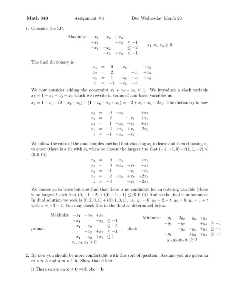
Math 340
Assignment #4
Due Wednesday March 23
1. Consider the LP:
Maximize −x1
−x1
−x1
−x2
−x2
−x2
+x3
−x3
+x3
≤ −1
≤ −2
≤ −1
x1 , x2 , x3 ≥ 0
The final dictionary is
x4
x2
x3
z
= 0 −x6
= 2
= 1 −x6
= −1 −x6
−x1
−x1
−x1
+x5
+x5
+x5
We now consider adding the constraint x1 + x2 + x3 ≤ 1. We introduce a slack variable
x7 = 1 − x1 − x2 − x3 which we rewrite in terms of non basic variables as
x7 = 1 − x1 − (2 − x1 + x5 ) − (1 − x6 − x1 + x5 ) = −2 + x6 + x1 − 2x5 . The dictionary is now
x4
x2
x3
x7
z
=
0 −x6
=
2
=
1 −x6
= −2 +x6
= −1 −x6
−x1
−x1
+x1
−x1
+x5
+x5
+x5
−2x5
We follow the rules of the dual simplex method first choosing x7 to leave and then choosing x1
to enter (there is a tie with x6 when we choose the largest t so that (−1, −1, 0) + t(1, 1, −2) ≤
(0, 0, 0))
x4 =
0 −x6
+x5
x2 =
0 +x6 −x7 −x5
x3 = −1
−x7 −x5
x1 =
2 −x6 +x7 +2x5
z = −3
−x7 −2x5
We choose x3 to leave but now find that there is no candidate for an entering variable (there
is no largest t such that (0, −1, −2) + t(0, −1, −1) ≤ (0, 0, 0)) And so the dual is unbounded.
In dual solution we seek is (0, 2, 0, 1) + t(0, 1, 0, 1), i.e. y1 = 0, y2 = 2 + t, y3 = 0, y4 = 1 + t
with z = −3 − t. You may check this in the dual as determined below:
primal:
Maximize −x1 −x2 +x3
−x1
−x3
−x1 −x2
−x2 +x3
x1 +x2 +x3
x1 , x2 , x3 ≥ 0
≤ −1
≤ −2
,
≤ −1
≤1
dual:
Minimize −y1 −2y2 −y3
−y1 −y2
−y2 −y3
−y1
+y3
y1 , y2 , y3 , y4 ≥ 0
+y4
+y4 ≥ −1
+y4 ≥ −1
+y4 ≥ −1
2. By now you should be more comfortable with this sort of question. Assume you are given an
m × n A and a m × 1 b. Show that either
i) There exists an x ≥ 0 with Ax = b
or
ii) There exists a y with AT y ≥ 0 and b · y < 0
but not both.
We begin by setting up a primal/dual pair of LP?s.
max
primal:
0·x
Ax = b
x≥0
min
dual:
b·y
AT y ≥ 0
y free
Please note that equations in one LP go to free variables in the dual and free variables go to
equations in the dual. We note that y = 0 is a feasible solution to the dual and so by the
Fundamental Theorem of Linear Programming, the dual either has an optimal solution or is
unbounded.
Case 1. Dual has an optimal solution
Let y∗ be an optimal dual solution. Then by Strong Duality Theorem, there is an optimal
solution x∗ to the primal. Then x∗ is feasible to the primal and so Ax = b and x ≥ 0. This
i) holds. Now 0 · x∗ = 0 and so by Weak Duality, any feasible solution to the dual, namely
any y satisfying AT y ≥ 0, has b · y ≥ 0. So ii) doesn?t hold.
Case 2. Dual is unbounded.
Thus there is a feasible solution to the dual, namely a y with AT y ≥ 0, satisfying b · y < 0
and so ii) holds. Now by Weak Duality, the dual being unbounded means there is no feasible
solution to the primal and so i) doesn’t hold.
Thus in either case we have one of i) and ii) holding but not both.
3. (from an old exam) We seek a minimum cost diet selected from the following three foods.
vitamins/100gms
calories/100gms
minimum (100gms)
food 1 food 2 food 3
13.23
18.4
36
100
125
139
10
10
8
cost $/100gm
3.00
5.00
8.00
We require a diet that has at least 760 units of vitamins and at least 3500 calories. The
minimums are stated in units of 100gms. We let the variable foodi refer to the amount of
food i purchased in units of 100gms. The input to LINDO is:
min 3food1+5food2+8food3
subject to
13.23food1+18.4food2+36food3>760
100food1+125food2+139food3>3500
food1>10
food2>10
food3>8
end
(from an old exam) a) There is a special on food 2 reducing the price to $4.10/100gms. This
would not change the your purchase strategy because the ‘current basis remains optimal’ and
so the current basic feasible solution B −1 b remains fixed even with a drop of $.91/100 gms.
A price reduction to $3.10 falls outside the range and one imagines the purchase strategy
would change
b) What is the marginal cost of 10 units of vitamins is 10 × .2222 which is $2.22. The chosen
diet as a whole has 760 units of vitamins and costs $178 and so the dollar cost of the whole
diet per 10 units of vitamins obtained is $178/76 = $2.34. The marginal cost is cheaper
(which is hardly surprising since the diet also has other constraints).
c) Integrality can be important in diet problems such as this if the foods come in integer
amounts (e.g. apples) but many foods are available in continuous amounts (bulk food bins)
and anyway can be divided at home into appropriate amounts. I expected some discussion
of the possibility that the variables for the foods were integral.
d) A linear inequality that expresses the requirement that at least 20% of the weight of the
purchased diet comes from food 2 is
f ood2 ≥ .2(f ood1 + f ood2 + f ood3)
which in LINDO input would become .2f ood1 − .8f ood2 + .2f ood3 ≤ 0.
4. (from an old exam) We have a gasoline blending problem where we may mix four gasoline
products x1 , x2 , x3 , x4 from 3 types of gas (gas1,gas2,gas3). The availability of the three gases
is given as a function of a parameter p:
Maximize 12.1x1 +8.3x2 +14.2x3 18.1x4
(= z)
(gas1)
2x1
+x2
+3x3
+6x4 ≤ 37 + 2p
x1 , x2 , x3 , x4
≥
0
(gas2)
3x1
+2x3
+x4
≤ 42 + p
(gas3)
x1
+4x2
+2x3
+x4
≤ 39 − 3p
We are interested in the value of the objective function z as a function of the parameter
p near p = 1. We make p a variable (and move it to the other side of the inequalities), and
make p free (allowing it to be negative). We also impose the somewhat arbitrary condition
p ≤ 1 and then use this constraint in our analysis. We send this off to LINDO. The LINDO
output will be useful for parts b),c).
a) When p = −37
, then the right hand side of the first inequality is 0 and we have 2x − 1 +
2
x2 + 3x3 + 6x4 = 0 and yet x1 , x2 , x3 , x4 ≥ 0. We deduce that x1 = x2 = x3 = x4 = 0 and so
z = 0 at optimality? For p < −37
we find that inequality 1 becomes 2x1 + x2 + 3x3 + 6x4 < 0
2
and yet x1 , x2 , x3 , x4 ≥ 0 which is a contradiction. Thus the LP is now infeasible.
b) For for p = 1, z = 230.8062 ? The slope of the graph of z as a function of p is rate of increase
of z as p increases. But p = 1 is imposed by the constraint PARAM p ≤ 1 (p wishes to increase
and so p = 1 at optimality) and the dual price for relaxing that constraint (and allowing p to
increase) is 2.5875. The range on p for which the slope valid is (1 − 2.269231, 1 + 3.045455).
c) Increasing p by ∆ (which should increase the objective function by ∆ times the dual price
for the 4th inequality) is like increasing the righthand side of the first inequality by 2∆, the
righthand side of the second inequality by ∆ and decreasing the righthand side of the third
inequality by 3∆ resulting in a predicted change in the z value by 2∆ times dual price for
constraint 1 and adding ∆ times dual price for constraint 2 and subtracting 3 ∆ times the
dual price for constraint 3. This yields the equality 2(2.525000)+1(1.868750)−3(1.443750) =
2.587500 after dividing by ∆. Another solution is to notice that in the dual, the constraint
associated with variable p in the primal, is −2y1 − y2 + 3y3 + y4 ≥ 0 and so since p > 0 we
have equality in this constraint by complementary slackness!
5. (from an old exam) We are running a factory and can produce products of three possible
types from four types of parts as follows.
part
part
part
part
1
2
3
4
profit $
product 1
3
4
5
4
product 2
5
6
8
7
product 3
2
2
3
4
21
35
15
available parts
286
396
440
396
We wish to choose our product mix to obtain maximum profit subject both to the limitations
on the inventory of available parts but also subject to the restriction that at most 50% of the
number of produced products can be of one type
The LINDO input/output on this page and the next page will be useful for parts a),b),c).
a)[2 marks] The marginal values of the four parts are 0, 0, 3, 1.545455.
b)[4 marks] Mr. Edison visits the factory and offers to make a remarkable new part that
substitutes for any of the four parts and will only charge $2 for each of these new parts.
Would you buy some? Yes, because the new part costs less than the marginal value for Part
3 and so you could substitute the new part for some number of Part 3’s. We can buy 24 new
parts and in essence have 24 more part 3’s and then make 3 × 24 more profit at an outlay of
2 × 24. We are using the right hand side ranges to see the range for which the marginal value
of 3 for Part 3 is valid.
c)[4 marks] The market for product 1 crashes and the profit drops to that of product 3.
Should you change your production? We see that the current basis remains the same and
hence the current production remains optimal even if we decrease the profit for Product 1
from $21 to $15 (allowable decrease is 6). Thus we need not change the production.
d)[4 marks] The marginal cost for the total parts that make up product 2 are 0 × 5 + 0 ×
9
× 7 = 34 11
which is less than the given profit of 35 per product 2. Normally
6 + 3 × 8 + 17
11
for a product in the basis you have the sum of the marginal values equal to the profit but
you are forgetting the 50% constraints. Increasing the production of Product 2 will violate
4
2
the PROD2<50 constraint and so we get an additional contribution of 11
× 0.5 = 11
to the
marginal cost of Product 2 which then yields equality of the marginal cost and the profit.
e) This question was not asked in the exam but was implicitly needed to explain the ‘discrepancy’ in d). The constraint PROD1<50
0.5 PROD1 - 0.5 PROD2 - 0.5 PROD3 < 0
can be rewritten as P ROD1 ≤ (1/2)(P ROD1+P ROD2+P ROD3) which was the constraint
that the number of Product 1 being produced is at most 50% of the total production.
6. (from an old exam) a) If tons of carbon removed per unit of strategy 1 is reduced from 15 to
14 what is now the total tons of carbon removed by an optimal strategy? The output says
the current basis and hence current solution remains optimal when we change 15 to 14 and
so tons of carbon removed drop by 1.5
b) We discover that the habitat damage is less crucial because new habitat for the endangered
species has been discovered on Pender Island. What is the benefit of allowing the habitat
damage to increase to 8.5 units from 8 units? We see that the right hand side can be increased
from 8 to 8.5. The marginal value of the habitat constraint is 26 so the change increases tons
carbon removed by (26) × (.50) = 13.
c) We are told that strategy 1 costs $5000 per unit, strategy 2 costs $6000 per unit and strategy
3 costs $10000 per unit. Is the cost in $ per ton of carbon removed less than $400 per ton for
our optimal strategy? This question has little to do with sensitivity analysis and more with
seeing if you can read the question. The total cost is (1.5) × 5000 + (3.5) × 10000 = 37, 500
and total tons carbon removed is 113.5. We readily compute that 37500/113.5 ≤ 400.
d) You are told of a new strategy of carbon removal using fertilizer to stimulate algae growth
that will require (per unit of new strategy) 100 units of capital, 100 units of labour, 2 units
space and 1 unit cost to habitat that will remove 19 tons of carbon. Should you investigate
further? The marginal values times the requirements are 100×0+100×0+2×0+1×26 = 26.
So the marginal cost of implementing (a unit) of the new strategy exceeds the profit (the
number of tons carbon removed) of 19. anges and seeWe would not explore this option.
e) A change in government has resulted in a new policy that we must choose 2 units of
strategy 1. How does this affect the number of tons of carbon removed? We must increase
strategy 1 from 1.5 to 2. We would start by considering the current politics constraint and
check the marginal value which is -63, namely increasing the rhs by 1 will cost 63 tons of
carbon removal. Thus increasing the rhs from 1.5 to 2 will cost 63 × (1/2) = 31.5 of tons of
carbon removed. We check the ranges and see that the marginal value is valid for increases
up to 1.1666. Political decisions can be expensive.