Summer 2015, NSERC USRA Report
Using Quasi Steady-State Approximation Methods to Analyze a
Non-linear Biological Motor Transport System
Timothy Small. Supervisors: Leah Keshet, Michael Ward
In the cell, two families of motors transport materials between the nucleus and periphery in
either direction. These kinesins and dyneins move in a similar fashion and can thus both be
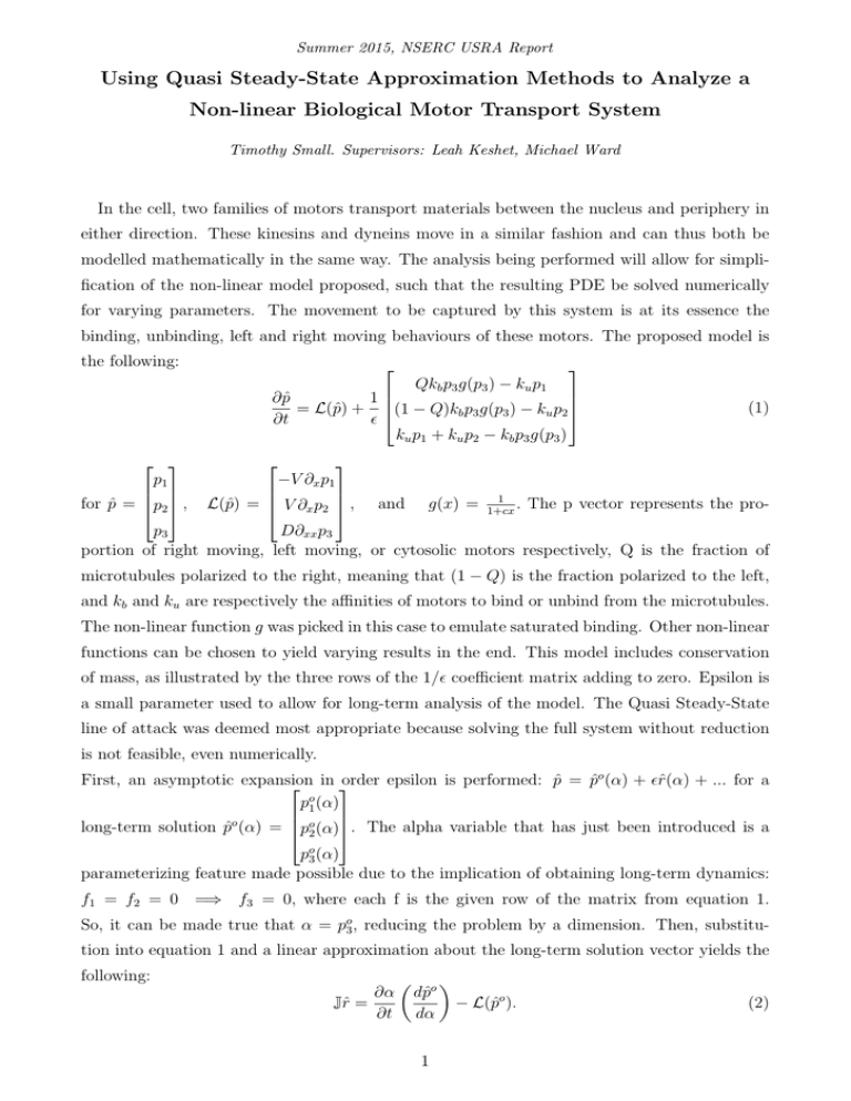
modelled mathematically in the same way. The analysis being performed will allow for simplification of the non-linear model proposed, such that the resulting PDE be solved numerically
for varying parameters. The movement to be captured by this system is at its essence the
binding, unbinding, left and right moving behaviours of these motors. The proposed model is
the following:

Qkb p3 g(p3 ) − ku p1


∂ p̂
1

= L(p̂) + 
(1
−
Q)k
p
g(p
)
−
k
p
b
3
3
u
2

∂t

ku p1 + ku p2 − kb p3 g(p3 )
(1)
 


p1
−V ∂x p1
 


 , L(p̂) =  V ∂x p2  , and g(x) = 1 . The p vector represents the profor p̂ = 
p
2
1+cx
 


p3
D∂xx p3
portion of right moving, left moving, or cytosolic motors respectively, Q is the fraction of
microtubules polarized to the right, meaning that (1 − Q) is the fraction polarized to the left,
and kb and ku are respectively the affinities of motors to bind or unbind from the microtubules.
The non-linear function g was picked in this case to emulate saturated binding. Other non-linear
functions can be chosen to yield varying results in the end. This model includes conservation
of mass, as illustrated by the three rows of the 1/ coefficient matrix adding to zero. Epsilon is
a small parameter used to allow for long-term analysis of the model. The Quasi Steady-State
line of attack was deemed most appropriate because solving the full system without reduction
is not feasible, even numerically.
First, an asymptotic expansion
order epsilon is performed: p̂ = p̂o (α) + r̂(α) + ... for a
 in 
po1 (α)


o

long-term solution p̂o (α) = 
p
(α)
 2 . The alpha variable that has just been introduced is a
po3 (α)
parameterizing feature made possible due to the implication of obtaining long-term dynamics:
f1 = f2 = 0 =⇒ f3 = 0, where each f is the given row of the matrix from equation 1.
So, it can be made true that α = po3 , reducing the problem by a dimension. Then, substitution into equation 1 and a linear approximation about the long-term solution vector yields the
following:
∂α
Jr̂ =
∂t
dp̂o
dα
1
− L(p̂o ).
(2)
Now, if a left eigenvector ψ T can be found for the Jacobian, equation 2 simplifies to just
∂α T dp̂o
(ψ
) = ψ T L(p̂o ).
∂t
dα
(3)
h
iT
Upon further inspection of the explicit Jacobian, ψ is simply the vector 1 1 1 . So, the
PDE
∂α
∂t
dpo1 dpo2 dpo3
+
+
dα
dα
dα
= −V ∂x po1 + V ∂x po2 + D∂xx po3
(4)
results.
The penultimate step to getting the final form PDE is computing the values of each of the poj
by using the prior stated condition that fj (po1 (α), po2 (α), po3 (α)) = 0 ∀j ∈ {1, 2, 3} for a long
time scale. The final step will be reducing the algebra. Solving in terms of α, where we have
mandated po3 = α yields that


γ1 α(1 + cα)−1


−1  ,
p̂o = 
γ
α(1
+
cα)
 2

α
where parameters γ1 =
Qkb
ku
and γ2 =
(1−Q)kb
ku
(5)
are created for ease of notation. Plugging this
back into equation 5 and simplifying all of the algebra leaves the following PDE:
∂α
∂α
∂ 2α
= V k1 (α)
+ k2 (α) 2 ,
∂t
∂x
∂x
for parameters k1 (α) =
B−A
,
A+B+1
k2 (α) =
D
,
A+B+1
A=
γ1
(1+cα)2
and B =
(6)
γ2
.
(1+cα)2
Solutions to this PDE will result in a definition for the parameter α and thus an expression
for the overall probability vector at long term steady-state. At this point, several tweaks can
be made to study more interesting aspects of this model, including changing the non-linear
function or making the Q parameter a function of space. These were explored in more detail in
the project but will not be written here due to spatial restraint. Suffice it to say that after the
fact, when the PDE from above was analyzed numerically with Matlab, some very interesting
and intuitively sensical graphs resulted. These graphs give a good idea of the behaviour of the
system after a long time has elapsed based on the parameters chosen, and therefore give insight
into certain aspects of the full evolution of the system.
The purpose of this project was not only to analyze long term solutions of one or two non-linear
models, but rather to demonstrate the capability of the Quasi Steady-State approximation
method to be applied to all sorts of interesting biological cases, as long as the conservation of
mass property is held. By reducing the initial problem, many interesting corollaries pop up
during the process, each of which leads to exploring side-problems that later rejoin in relevance
to the main analysis. Therefore, this project as a whole was structured to not only look at the
narrow base case of the model, but to also lead to other interesting observations that support
the claim that mathematical models work both robustly and flexibly in explaining biological
phenomena.
2