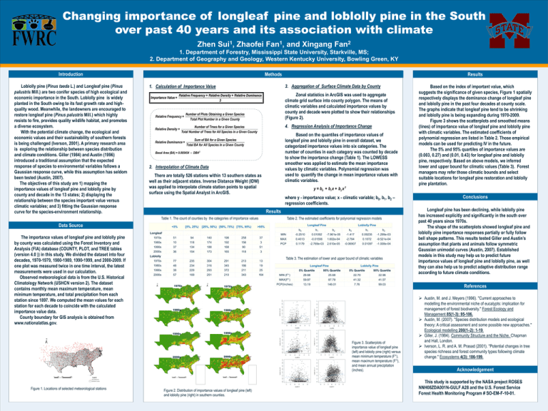
Changing importance of longleaf pine and loblolly pine in the South
over past 40 years and its association with climate
Zhen Sui1, Zhaofei Fan1, and Xingang Fan2
1. Department of Forestry, Mississippi State University, Starkville, MS;
2. Department of Geography and Geology, Western Kentucky University, Bowling Green, KY
Introduction
Loblolly pine (Pinus taeda L.) and Longleaf pine (Pinus
palustris Mill.) are two conifer species of high ecological and
economic importance in the South. Loblolly pine is widely
planted in the South owing to its fast growth rate and highquality wood. Meanwhile, the landowners are encouraged to
restore longleaf pine (Pinus palustris Mill.) which highly
resists to fire, provides quality wildlife habitat, and promotes
a diverse ecosystem.
With the potential climate change, the ecological and
economic values and their sustainability of southern forests
is being challenged (Iverson, 2001). A primary research area
is exploring the relationship between species distribution
and climate conditions. Giller (1984) and Austin (1996)
introduced a traditional assumption that the expected
response of species to environmental variables follows a
Gaussian response curve, while this assumption has seldom
been tested (Austin, 2007).
The objectives of this study are 1) mapping the
importance values of longleaf pine and loblolly pine by
county and decade in the 13 states; 2) displaying the
relationship between the species important value versus
climatic variables; and 3) fitting the Gaussian response
curve for the species-environment relationship.
Methods
3. Aggregation of Surface Climate Data by County
1. Calculation of Importance Value
Importance Value =
Zonal statistics in ArcGIS was used to aggregate
climate grid surface into county polygon. The means of
climatic variables and calculated importance values by
county and decade were plotted to show their relationships
(Figure 2).
Relative Frequency + Relative Density + Relative Dominance
3
Relative Frequency =
Number of Plots Obtaining a Given Species
Total Plot Number in a Given County
4. Regression Analysis of Importance Change
Number of Trees for a Given Species
Relative Density =
Total Number of Trees for All Species in a Given County
Relative Dominance =
Results
Based on the quantiles of importance values of
longleaf pine and loblolly pine in overall dataset, we
categorized importance values into six categories. The
number of counties in each category was counted by decade
to show the importance change (Table 1). The LOWESS
smoother was applied to estimate the mean importance
values by climatic variables. Polynomial regression was
used to quantify the change in mean importance values with
climatic variables.
Sum of BA for a Given Species
Total BA for All Species In a Given County
Basal Area (BA) = 0.005454 × DBH 2
2. Interpolation of Climate Data
There are totally 526 stations within 13 southern states as
well as their adjacent states. Inverse Distance Weight (IDW)
was applied to interpolate climate station points to spatial
surface using the Spatial Analyst in ArcGIS.
y = b0 + b1 x + b2 x 2
where y - importance value; x - climatic variable; b0, b1, b2 –
regression coefficients.
Results
Table 1. The count of counties by the categories of importance values
Data Source
The importance values of longleaf pine and loblolly pine
by county was calculated using the Forest Inventory and
Analysis (FIA) database (COUNTY, PLOT, and TREE tables
(version 4.0 )) in this study. We divided the dataset into four
decades, 1970-1979, 1980-1989, 1990-1999, and 2000-2009. If
one plot was measured twice in one time interval, the latest
measurements were used in our calculation.
Observed meteorological data is from the U.S. Historical
Climatology Network (USHCN version 2). The dataset
contains monthly mean maximum temperature, mean
minimum temperature, and total precipitation from each
station since 1897. We computed the mean values for each
station for each decade to coincide with the calculated
importance value data.
County boundary for GIS analysis is obtained from
www.nationalatlas.gov.
<5%
[25%, 50%) [50%, 75%) [75%, 95%)
Longleaf Pine
>95%
Longleaf
Loblolly Pine
b0
b1
b2
b0
b1
b2
MIN
-0.2510
0.01092
-7.961e-05
-1.417
0.09235
-1.299e-03
1970s
51
94
140
198
258
37
MAX
0.4013
-0.01556
1.602e-04
-2.794
0.1072
-9.521e-04
1980s
10
118
174
192
156
3
PCP
0.1179
-2.769e-03
2.610e-05
-0.06907
0.01097
-1.008e-04
1990s
37
134
188
168
90
51
2000s
36
154
173
165
118
3
1970s
77
235
304
291
213
13
1980s
48
234
316
345
186
19
1990s
38
229
293
372
211
25
2000s
57
169
251
210
343
164
Loblolly
1970s
1970s
1980s
1980s
1990s
1990s
2000s
Figure 1. Locations of selected meteorological stations
[5%, 25%)
Table 2. The estimated coefficients for polynomial regression models
2000s
Figure 2. Distribution of importance values of longleaf pine (left)
and loblolly pine (right) in southern counties.
Table 3. The estimation of lower and upper bound of climatic variables
Longleaf Pine
Loblolly Pine
5% Quartile
95% Quartile
5% Quartile
95% Quartile
MIN (F°)
29.68
25.68
22.70
22.96
MAX(F°)
59.87
87.79
41.32
41.57
PCP(Inches)
13.19
146.01
7.76
99.03
Figure 3. Scatterplots of
importance value of longleaf pine
(left) and loblolly pine (right) versus
mean minimum temperature (F°),
mean maximum temperature (F°),
and mean annual precipitation
(inches).
Based on the index of important value, which
suggests the significance of given species, Figure 1 spatially
respectively displays the dominance change of longleaf pine
and loblolly pine in the past four decades at county scale.
The graphs indicate that longleaf pine tend to be shrinking
and loblolly pine is being expanding during 1970-2009.
Figure 3 shows the scatterplots and smoothed means
(lines) of importance value of longleaf pine and loblolly pine
with climatic variables. The estimated coefficients of
polynomial regression are listed in Table 2. Those empirical
models can be used for predicting IV in the future.
The 5% and 95% quartiles of importance values are
(0.003, 0.27) and (0.01, 0.43) for longleaf pine and loblolly
pine, respectively. Based on above models, we inferred
lower and upper bound for climatic values (Table 3). Forest
managers may refer those climatic bounds and select
suitable locations for longleaf pine restoration and loblolly
pine plantation.
Conclusions
Longleaf pine has been declining, while loblolly pine
has increased explicitly and significantly in the south over
past 40 years since 1970s.
The shape of the scatterplots showed longleaf pine and
loblolly pine importance responses partially or fully follow
bell shape patterns. This results tested Giller and Austin’s
assumption that plants and animals follow symmetric
Gaussian unimodal curves (Austin, 2007). Established
models in this study may help us to predict future
importance values of longleaf pine and loblolly pine, as well
they can also help us to predict adaptive distribution range
according to future climate conditions.
References
 Austin, M. and J. Meyers (1996). "Current approaches to
modelling the environmental niche of eucalypts: implication for
management of forest biodiversity." Forest Ecology and
Management 85(1-3): 95-106.
 Austin, M. (2007). "Species distribution models and ecological
theory: A critical assessment and some possible new approaches."
Ecological modelling 200(1–2): 1-19.
 Giller, J. (1984). Community Structure and the Niche. Chapman
and Hall, London.
 Iverson, L. R. and A. M. Prasad (2001). "Potential changes in tree
species richness and forest community types following climate
change." Ecosystems 4(3): 186-199.
Acknowledgement
This study is supported by the NASA project ROSES
NNH08ZDA001N-GULF A28 and the U.S. Forest Service
Forest Health Monitoring Program # SO-EM-F-10-01.