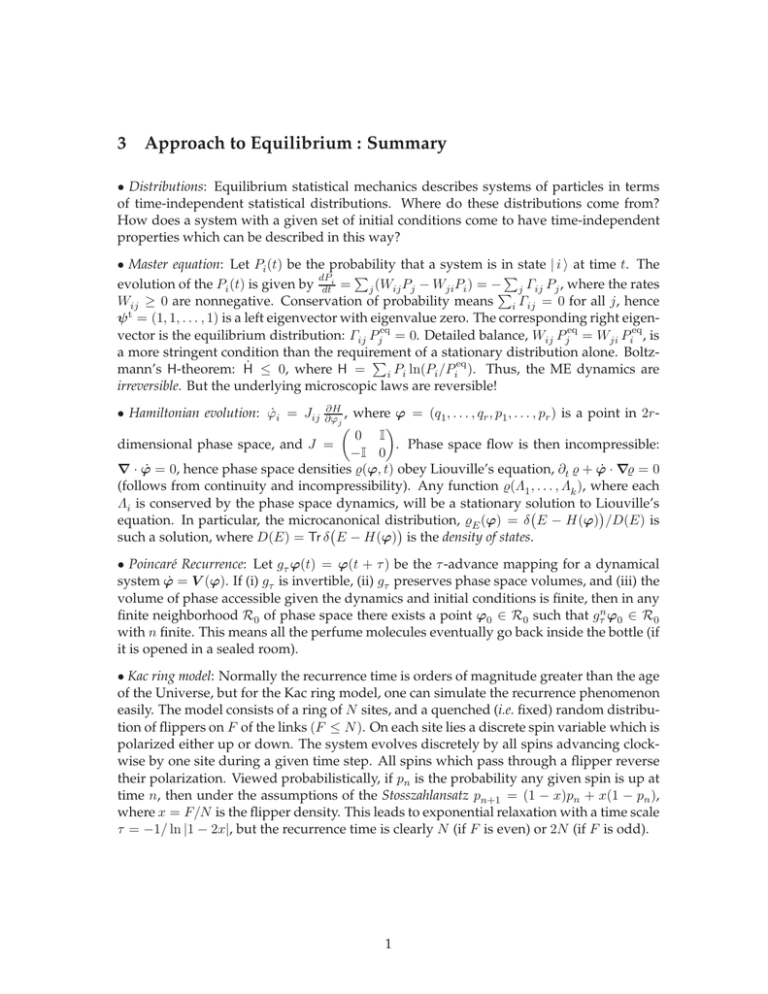
3 Approach to Equilibrium : Summary
• Distributions: Equilibrium statistical mechanics describes systems of particles in terms
of time-independent statistical distributions. Where do these distributions come from?
How does a system with a given set of initial conditions come to have time-independent
properties which can be described in this way?
• Master equation: Let Pi (t) be the probability that a system is in state | i i at time t. The
P
P
dP
evolution of the Pi (t) is given by dti = j (Wij Pj − Wji Pi ) = −P j Γij Pj , where the rates
Wij ≥ 0 are nonnegative. Conservation of probability means i Γij = 0 for all j, hence
ψ t = (1, 1, . . . , 1) is a left eigenvector with eigenvalue zero. The corresponding right eigenvector is the equilibrium distribution: Γij Pjeq = 0. Detailed balance, Wij Pjeq = Wji Pieq , is
a more stringent condition than the requirement
of a stationary distribution alone. BoltzP
eq
mann’s H-theorem: Ḣ ≤ 0, where H =
P
ln(P
i /Pi ). Thus, the ME dynamics are
i i
irreversible. But the underlying microscopic laws are reversible!
∂H
∂ϕj ,
where ϕ = (q1 , . . . , qr , p1 , . . . , pr ) is a point in 2r
0 I
dimensional phase space, and J =
. Phase space flow is then incompressible:
−I 0
∇ · ϕ̇ = 0, hence phase space densities ̺(ϕ, t) obey Liouville’s equation, ∂t ̺ + ϕ̇ · ∇̺ = 0
(follows from continuity and incompressibility). Any function ̺(Λ1 , . . . , Λk ), where each
Λi is conserved by the phase space dynamics, will be a stationary solution to Liouville’s
equation. In particular, the microcanonical distribution,
̺E (ϕ) = δ E − H(ϕ) /D(E) is
such a solution, where D(E) = Tr δ E − H(ϕ) is the density of states.
• Hamiltonian evolution: ϕ̇i = Jij
• Poincaré Recurrence: Let gτ ϕ(t) = ϕ(t + τ ) be the τ -advance mapping for a dynamical
system ϕ̇ = V (ϕ). If (i) gτ is invertible, (ii) gτ preserves phase space volumes, and (iii) the
volume of phase accessible given the dynamics and initial conditions is finite, then in any
finite neighborhood R0 of phase space there exists a point ϕ0 ∈ R0 such that gτn ϕ0 ∈ R0
with n finite. This means all the perfume molecules eventually go back inside the bottle (if
it is opened in a sealed room).
• Kac ring model: Normally the recurrence time is orders of magnitude greater than the age
of the Universe, but for the Kac ring model, one can simulate the recurrence phenomenon
easily. The model consists of a ring of N sites, and a quenched (i.e. fixed) random distribution of flippers on F of the links (F ≤ N ). On each site lies a discrete spin variable which is
polarized either up or down. The system evolves discretely by all spins advancing clockwise by one site during a given time step. All spins which pass through a flipper reverse
their polarization. Viewed probabilistically, if pn is the probability any given spin is up at
time n, then under the assumptions of the Stosszahlansatz pn+1 = (1 − x)pn + x(1 − pn ),
where x = F/N is the flipper density. This leads to exponential relaxation with a time scale
τ = −1/ ln |1 − 2x|, but the recurrence time is clearly N (if F is even) or 2N (if F is odd).
1
• Ergodicity and mixing: A dynamical system is ergodic if
1
f (ϕ) T = lim
T →∞ T
ZT
Tr f (ϕ) δ E − H(ϕ)
= f (ϕ) S .
dt f ϕ(t) =
Tr δ E − H(ϕ)
0
This means long time averages are equal to phase space averages. This does not necessarily
mean that the phase space distribution will converge to the microcanonical distribution.
A stronger condition, known as mixing, means that the distribution spreads out ’evenly’
over the phase space hypersurface consistent with all conservation laws. Thus, if g is a
phase space map, and if ν(A) ≡ DA (E)/D(E) is the fraction of the energy hypersurface
(assume no conserved quantities other than H = E) contained in A, then g is mixing if
limn→∞ ν (gn A ∩ B) = ν(A) ν(B). An example of a mixing map on a two-dimensional
torus is the Arnold ’cat map’,
′ q
1 1
q
=
mod Z2 .
p′
1 2
p
• Thermalization of quantum systems: This is a current research topic. One proposal, due to
Deutsch (1991) and Srednicki (1994) is the eigenstate thermalization hypothesis (ETH). This
says that thermal information is encoded in each eigenstate, such that if Eα ∈ [E, E + ∆E],
then
h Ψα | A | Ψα i = hAiEα ,
i.e. the expectation value of some local, translationally-invariant, few-body operator A in
the state | Ψα i, is given by its average over a small energy window containing Eα . If this
is the case, then so long as we prepare an initial state such that the spread of energies is
within ∆E of some value E, where ∆E ≪ E − E0 with E0 the ground state energy, then
hAiT = hAiE , and time averages become energy averages. Equivalently, the reduced density
matrix ρS corresponding to a system S which is a subset of a universe U , with W ∪S = U (W
is the ’world’), is a thermal density matrix: ρS = ZS−1 e−β ĤS , where ĤS is the Hamiltonian
restricted to S, and with temperature fixed by the requirement Tr(ρS ĤS ) = E · (VS /VU ),
where the last factor is a ratio of volumes. ETH does not hold for so-called integrable models with an extensive number of independent conserved quantities. But it has been shown,
both perturbatively as well as numerically, to hold for certain model nonintegrable systems. An interesting distinction between classical and quantum thermalization: in the
quantum case, time evolution does not create the thermal state. Rather, it reveals the thermal distribution which is encoded in each eigenstate after sufficient time that dephasing has
occurred and all correlations between the different wavefunction expansion coefficients is
lost.
2