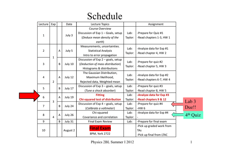
Schedule
Lecture Exp
Date
B
July 24
A
July 26
B
July 31
Lecture Topics
Course Overview
Discussion of Exp 1 – Goals, setup
(Deduce mean density of the
earth)
Measurements, uncertainties.
Statistical Analysis
Intro to error propagation
Discussion of Exp 2 – goals, setup
(Deduction of mass distribution)
Histograms & distributions
The Gaussian Distribution,
Maximum likelihood,
Rejected data, Weighted mean
Discussion of Exp 3 – goals, setup
(Tune a shock absorber)
Fitting
Chi-squared test of distribution
Discussion of Exp 4 – goals, setup
(Calibrate a voltmeter)
Chi-squared
Covariance and correlation
Final Exam Review
August 2
Final Exam
1
July 3
2
A
July 5
3
B
July 10
4
A
July 12
5
B
July 17
6
A
July 19
1
2
3
7
8
9
10
4
Assignment
Lab: -Prepare for Quiz #1
Taylor: -Read chapters 1-3, HW 1
Lab: -Analyze data for Exp #1
Taylor: -Read chapter 4, HW 2
Lab: -Prepare for quiz #2
Taylor: -Read chapter 5, HW 3
Lab: -Analyze data for Exp #2
Taylor: -Read chapters 6-7, HW 4
Lab:
Taylor:
Lab:
Taylor:
Lab:
Taylor:
Lab:
Taylor:
Lab:
8PM, York 2722
Physics 2BL Summer I 2012
-Prepare for quiz #3
-Read chapter 8, HW 5
-Analyze data for Exp #3
-Read chapters 9 & 12
-Prepare for quiz #4
-HW 6
-Analyze data for Exp #4
-Prepare for final exam
-Pick up graded work from
TAs
-Pick up final from LTAC
Lab 3
Due!!
4th Quiz
1
Introduction to Linear Least
Squares Fitting
χ2 analysis
Lecture # 6
Physics 2BL
Summer Session I 2012
Physics 2BL Summer I 2012
2
Lecture #6:
• Issues from experiment 3?
– Tuesday you will need to turn in your lab
notebook/report before the end of lab
– Start it at home! (may need to retake data)
• Experiment 3 writeup
• Recap:
– Principle of Maximum Likelihood
• Linear Least Squares fitting
• Chi-Squared
• Homework
Physics 2BL Summer I 2012
3
Exp 3 - Measurements
• Make sure to include ALL
measurements (with
uncertainties) in the same
section
∆x
• Thickness of the mass
?
– Did you measure the correct
thickness?
– If not, how does this affect
your lab results?
Physics 2BL Summer I 2012
4
Exp 3 - Graphs
• Graphs of velocity vs drop
height
– Only for 4 and 5 holes open
– Discuss trends and their meaning!
– Answer questions: “Will the mass
reach terminal velocity for 6 or 7
holes open? Etc…”
• Graph of b vs # holes open
– draw smooth line thru data and plot
bcrit as a horizontal line
– Estimate # holes open for critical
damping
Physics 2BL Summer I 2012
5
Exp 3 - Calculations
• Make sure to do every part of the rubric
• Calculate kspring with uncertainty (using the period)
• Calculate kby-eye with uncertainty (using ∆t* at
critical damping)
b
2
bcrit = 2 mk
– According to model
mg
b
=
– Terminal velocity
vt
∆x
– Kinematics vt =
k=
k=
2
mg
2
4vt
∆t *
kby −eye
crit
4m
 g∆t * 
= m

 2∆x 
2
• How did you know you reached critical damping?
• Calculate a weighted mean for k (with uncertainty,
as usual)
Physics 2BL Summer I 2012
6
Exp 3 - Conclusion
• Comparison of kspring and kby-eye using tscore
– Determine the level at which the 2 values are
discrepant
• Discuss error:
– Specific sources of random or systematic error
– How you reduced random/systematic error
– How can you improve?
Physics 2BL Summer I 2012
7
Recap
• Principle of maximum likelihood
1
− ( x − X )2
PX ,σ ( x ) =
e
σ 2π
2σ 2
– L = P(x1)P(x2)…P(xN)
– Prove that the mean maximizes the
X = x δX = σ x
likelihood when errors are equal
– Prove that the weighted mean
maximizes the likelihood when errors
xi wi
are different
1
∑
X = xwav =
δX = σ wav =
∑ wi
∑ wi
• Minimize chi-squared
χ
2
N
=
∑
i =1
 xi − X

 σi
wi =



2
Physics 2BL Summer I 2012
1
σ i2
=
1
(δxi )2
8
Fitting Data
• We often fit data using a maximum likelihood
Bx + Cx + …
method to determine parameters. yy == AA +cos(Bx
+ C) + D
• For errors which are “Normal”, we can just
minimize the χ2.
2
2
∂χ
=0
∂X
• We will use this method to fit straight lines to data.
• More complex functions can be fit the same way.
To determine a straight line we need 2
parameters. How do we get 2 equations?
Physics 2BL Summer I 2012
9
LINEAR FIT: y(x) = A + Bx
minimize
30
Σ
[yj-(A+Bxj)] 2
True value, X(xj)
20
y((x)
y4-(A+Bx4)
y3-(A+Bx3)
10
Assumptions:
δxj << δyj ; δxj = 0
yj – normally distributed
σj: same for all yj
0
0
5
10
15
x
20
Physics 2BL Summer I 2012
25
10
Linear Fit
• Determine A and B by minimizing the square of the
deviations between your measurements and the
“theory”.
Minimize → ∑ (y i − (A + Bx i ))
2
i
Measurements
“Theory”
Physics 2BL Summer I 2012
11
LINEAR FIT: y(x) = A + Bx
2


(
)
−
y
−
y
1
j
true
Pr ob(y j )∝
exp 

2
σy
2σ y


30
y(x)
20
10
0
0
5
10
15
20
25
2

− (y j − A − Bx j ) 
1
=
exp 

2
σy
2σ y


Pr ob(y1 , y 2 ,... y N ) = Pr ob(y1 )× Pr ob(y 2 )× ... × Pr ob(y N )
x
2
 − (y1 − A − Bx1 )2
− (y N − A − Bx N ) 
= N exp 
+ ... +

2
2
σ
2σ y
2σ y


N − (y − A − B )2
1
1
1
j
j
= N exp ∑
= N
2
N (y − A − B )2
σ
σ
σ
2
j =1
y
j
exp ∑ j
2σ y2
j =1
2
[y
-(A+Bx
)]
Best estimates of A&B
max Prob(y1…yN)
min
j
j
1
Physics 2BL Summer I 2012
Σ
12
LINEAR FIT: y(x) = A + Bx
30
To determine A & B need to
[yj-(A+Bxj)]
y(x)
Σ
minimize:
20
2
10
0
0
5
10
15
20
25
x
∂ ∑ (y j − A − Bx j )
2
∂A
∂ ∑ (y j − A − Bx j )
=0
2
∂B
=0
A=
2
x
∑ j ∑ yj − ∑ xj∑ xj yj
B=
N ∑ x − (∑ x j )
2
j
2
N∑ xj y j − ∑ xj ∑ y j
N ∑ x − (∑ x j )
2
j
Sometime denote:
∆ = N∑x −
2
Physics 2BL Summer I 2012
2
(∑ x)
2
13
Deducing Errors
• As in the case of experiment 2, sometimes we can’t
estimate the errors too well before-hand.
• In such cases we compared many measurements to the
mean and computed the RMS.
• In this case we will compare to deviations from a line
– 2 Dimension “extension”.
σy
2
N
1
2
( yi − A − Bxi )
=
∑
N − 2 i =1
Note that now we use (N - 2)
because we have fit 2 parameters.
Where did we use (N-1)?
Physics 2BL Summer I 2012
14
Motivation for the (N-2)
• Averages (1 parameter)
– no deviations from one point
1 N
2
(xi − x )
σx =
∑
N − 1 i =1
– “reduced” deviations from two (or more)
points
• Straight lines (2 parameters)
– no deviations from two points
1 N
2
(
)
σy =
y
−
A
−
Bx
∑
i
i
N − 2 i =1
– “reduced” deviations form three (or
more) points
Physics 2BL Summer I 2012
15
Uncertainties in y, A, and B
σy =
1 N
2 uncertainty in the measurement of y
( yi − A − Bxi ) (If we already have an independent
∑
N − 2 i =1
estimate of the uncertainty in y , …, y we
1
σA =σy
σB = σ y
expect this estimate to compare with σy)
2
x
∑
uncertainties in the constants A and B
given by error propagation in terms
of uncertainties in y1, … , yN
∆
N
∆
 ∂A 
σ A = ∑  σ y 
i =1  ∂yi

N
Where
∆ = N∑x −
2
N
(∑ x)
2
2
Physics 2BL Summer I 2012
16
How good is my fit? χ2 test for fit
 y j − f (x j )
χ = ∑

σy
j =1 


N
2
Roughly speaking:
~ N it’s a good fit
>>N it’s a Bad fit
2
30
y(x))
20
10
How good is the agreement
between theory and data?
0
0
5
10
15
20
25
x
Physics 2BL Summer I 2012
17
χ2 test for fit
 y j − f (x j )
2
χ = ∑

σy
j =1 


N
30
2
Define reduced χ2
χ
2
~
χ =
d
2
20
y(x))
# of degrees of
freedom
d=N-c
10
# of data
points
0
0
5
10
15
20
25
# of parameters
calculated from
data (constraints)
x
Physics 2BL Summer I 2012
18
The Chi-Squared Test
• Minimized χ2 (maximize likelihood) to fit data
• Use χ2 to determine if we used a good
hypothesis
• Reduced χ2 will be nearly 1 for good fit
(χ2 ~ d)
• Use χ2 per degree of freedom to compute a
probability that the data are consistent with the
hypothesis (table D)
• Probability from table = confidence level
 y j − f (x j )
χ = ∑

σy
j =1 


N
2
2
d=N-c
χ~ 2 =
(
χ2
d
2
Pd χ~ 2 ≥ χ~0
)
Disagreement is “significant”
if probability is less than 5%
Disagreement is “highly
significant” if probability is
less than 1%
Physics 2BL Summer I 2012
20
Summary - Fitting
• You have a set of measurements and a hypothesis that
relates them.
• The hypothesis has some unknown parameters that you
want to determine.
• You “fit” for the parameters by maximizing the odds of all
measurements being consistent with your hypothesis.
• Evaluate your fit based on the goodness of fit.
Physics 2BL Summer I 2012
22
The Chi-Squared Test for a distribution
• You take N measurements of some parameter x which you
believe should be distributed in a certain way (e.g., based
on some hypothesis).
• You divide them into n bins (k=1,2,...,n) and count the
number of observations that fall into each bin (Ok).
• You also calculate the expected number of measurements
(Ek), in the same bins, based on some hypothesis. Uncertainties
in Counting:
2
• Calculate:
n
Ok − Ek )
(
2
q = N (integer #)
δ (Ek ) = Ek
χ =∑
i =1
Ek
• If χ2 < n, then the agreement between the
δq = N
observed and expected distributions is acceptable.
• If χ2 >> n, there is significant disagreement.
Physics 2BL Summer I 2012
23
Degrees of Freedom for a distribution
• Number of degrees of freedom, d = number of bins, n,
minus the number of parameters computed from the data
and used in the calculation.
• d = n ‐ c,
– Where c is the number of parameters that were calculated in order
to compute the expected distribution, Ek.
– It can be shown that the expected average value of χ2 is d.
• Therefore, we define “reduced chi‐squared”:
‐
χ% 2 =
χ2
nd.o.f.
• If the reduced chi-squared is ~1, there is no reason to doubt
the expected distribution.
Physics 2BL Summer I 2012
24
Homework
• Finish Experiment # 3
• If you need to retake data, visit Chris’s
office hours (M 10am-12pm)
• Read Taylor chapters 9 & 12
• Start analysis so you finish lab 3 on time!
Physics 2BL Summer I 2012
26