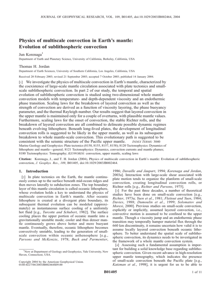
JOURNAL OF GEOPHYSICAL RESEARCH, VOL. 109, B01405, doi:10.1029/2003JB002464, 2004
Physics of multiscale convection in Earth’s mantle:
Evolution of sublithospheric convection
Jun Korenaga1
Department of Earth and Planetary Science, University of California, Berkeley, California, USA
Thomas H. Jordan
Department of Earth Sciences, University of Southern California, Los Angeles, California, USA
Received 20 February 2003; revised 21 September 2003; accepted 7 October 2003; published 14 January 2004.
[1] We investigate the physics of multiscale convection in Earth’s mantle, characterized by
the coexistence of large-scale mantle circulation associated with plate tectonics and smallscale sublithospheric convection. In part 2 of our study, the temporal and spatial
evolution of sublithospheric convection is studied using two-dimensional whole mantle
convection models with temperature- and depth-dependent viscosity and an endothermic
phase transition. Scaling laws for the breakdown of layered convection as well as the
strength of convection are derived as a function of viscosity layering, the phase buoyancy
parameter, and the thermal Rayleigh number. Our results suggest that layered convection in
the upper mantle is maintained only for a couple of overturns, with plausible mantle values.
Furthermore, scaling laws for the onset of convection, the stable Richter rolls, and the
breakdown of layered convection are all combined to delineate possible dynamic regimes
beneath evolving lithosphere. Beneath long-lived plates, the development of longitudinal
convection rolls is suggested to be likely in the upper mantle, as well as its subsequent
breakdown to whole mantle-scale convection. This evolutionary path is suggested to be
INDEX TERMS: 3040
consistent with the seismic structure of the Pacific upper mantle.
Marine Geology and Geophysics: Plate tectonics (8150, 8155, 8157, 8158); 8120 Tectonophysics: Dynamics of
lithosphere and mantle—general; 8121 Tectonophysics: Dynamics, convection currents and mantle plumes;
8180 Tectonophysics: Tomography; KEYWORDS: convection, upper mantle, scaling laws
Citation: Korenaga, J., and T. H. Jordan (2004), Physics of multiscale convection in Earth’s mantle: Evolution of sublithospheric
convection, J. Geophys. Res., 109, B01405, doi:10.1029/2003JB002464.
1. Introduction
[2] In plate tectonics on the Earth, the mantle continuously comes up to the surface beneath mid-ocean ridges and
then moves laterally to subduction zones. The top boundary
layer of this mantle circulation is called oceanic lithosphere,
whose evolution holds a key to understand the physics of
multiscale convection in Earth’s mantle. After oceanic
lithosphere is created at a divergent plate boundary, its
subsequent thermal evolution can be modeled (approximately) as instantaneous surface cooling of a uniformly
hot fluid [e.g., Turcotte and Schubert, 1982]. The surface
cooling places the upper portion of oceanic mantle into a
gravitationally unstable mode; cooler and thus denser mantle continuously grows above hotter and more buoyant
mantle. Eventually, therefore, oceanic lithosphere becomes
convectively unstable, leading to the generation of smallscale convection within oceanic asthenosphere [e.g.,
Parsons and McKenzie, 1978; Buck and Parmentier,
1
Now at Department of Geology and Geophysics, Yale University, New
Haven, Connecticut, USA.
Copyright 2004 by the American Geophysical Union.
0148-0227/04/2003JB002464$09.00
1986; Davaille and Jaupart, 1994; Korenaga and Jordan,
2003a]. Interaction with large-scale shear associated with
plate motion tends to organize the planform of small-scale
convection, creating longitudinal convection rolls, or
Richter rolls [e.g., Richter and Parsons, 1975].
[3] For the past three decades, a number of theoretical
studies have been done on small-scale convection [e.g.,
Richter, 1973a; Yuen et al., 1981; Fleitout and Yuen, 1984;
Davies, 1988; Dumoulin et al., 1999; Solomatov and
Moresi, 2000]. Previous studies on small-scale convection,
explicitly or implicitly, assumed layered convection, i.e.,
convective motion is assumed to be confined to the upper
mantle. Though a viscosity jump and an endothermic phase
transition may temporally hamper material flux through the
660 km discontinuity, it remains uncertain how valid it is to
assume locally layered convection beneath oceanic lithosphere. To better understand the spatial scale of sublithospheric convection, its dynamics needs to be investigated in
the framework of a whole mantle convection system.
[4] Assessing such a fundamental assumption is important for building a solid knowledge base regarding sublithospheric convection. Given recent advance in high-resolution
upper mantle tomography, which indicates the presence
of small-scale convection beneath the Pacific plate [e.g.,
Katzman et al., 1998], it is urgent for us to be able to
B01405
1 of 11
B01405
KORENAGA AND JORDAN: EVOLUTION OF SUBLITHOSPHERIC CONVECTION
Figure 1. Schematic diagram of possible evolution of
sublithospheric convection in oceanic mantle [after
Korenaga and Jordan, 2003a].
predict theoretically the dynamic state of oceanic upper
mantle. Such capability will with no doubt facilitate productive feedback between theory and observation. Given
uncertainties regarding the physical and rheological properties of the mantle, obtaining a scaling law that can handle a
wide range of parameters is essential. The purpose of this
paper is, therefore, to establish scaling laws for the dynamics of a whole mantle system that exhibits both large-scale
mantle circulation and small-scale convection, on the basis
of a large number of 2-D numerical calculations.
[5] This paper focuses on the potential evolution of sublithospheric, so-called ‘‘small-scale’’ convection (Figure 1).
Note that the very first phase, i.e., the onset of convection,
has already been studied by Korenaga and Jordan [2003a].
The temporal variation of the spatial scale of sublithospheric
convection is studied by 2-D convection models with
temperature- and depth-dependent viscosity and an endothermic phase transition. The concept of morphological
similarity is introduced here. A scaling law for the breakdown of layered convection to whole mantle convection is
derived for a transient cooling problem with a range of
viscosity layering and phase boundary buoyancy. Finally,
combining with other scaling laws for sublithospheric
convection derived in previous studies, we discuss possible
dynamic regimes expected beneath oceanic plates.
2. Spatial Evolution of Sublithospheric
Convection
[6] The spatial scale of sublithospheric convection has
long been assumed to be small compared to global mantle
circulation (hence sublithospheric convection and small-
B01405
scale convection are often used interchangeably). This is
equivalent to assuming that sublithospheric convection is
confined in the upper mantle, but how valid is this assumption? In other words, can the mantle be layered for sublithospheric convection? Though there has been extensive
discussion on the possibility of layered mantle convection
based on numerical modeling [e.g., Christensen and Yuen,
1984; Machetel and Weber, 1991; Tackley et al., 1993;
Puster and Jordan, 1997], its focus has been mostly on
global mantle circulation, and much less attention has been
paid for the layering of sublithospheric convection. There
are at least two potential mechanisms in favor of layering:
depth-dependent viscosity and endothermic phase transition. Geophysical observations suggest that the lower mantle is probably 30 times more viscous than the upper
mantle [e.g., Hager et al., 1985; Forte and Mitrovica, 1996;
Simons and Hager, 1997]. Viscosity layering, of course,
does not completely prevent cold downwelling from the
base of lithosphere to sink into the lower mantle. It simply
increases the timescale for penetration, which may result in
the temporary layering of sublithospheric convection.
[7] An endothermic phase transition between g-spinel and
perovskite + magnesiowüstite that occurs at around 660 km
depth [e.g., Ito et al., 1990], on the other hand, provides
positive buoyancy due to the deformation of the phase
boundary, which may partially cancel the negative thermal
buoyancy. Whole mantle convection models have consistently demonstrated that a reasonable value of the Clapeyron
slope (i.e., 2 to 3 MPa K1) leads to intermittent layered
convection [e.g., Machetel and Weber, 1991; Tackley et al.,
1993; Honda et al., 1993; Solheim and Peltier, 1994], except
at very high Rayleigh numbers, with which complete layering is possible [e.g., Yuen et al., 1994]. The strength of a
phase boundary in stationary state convection is the main
interest of these convection studies. Previous studies on the
relation between transient convection and phase change
dynamics have been limited mostly to the interaction of an
upwelling plume with an endothermic phase boundary [e.g.,
Nakakuki et al., 1994; Schubert et al., 1995; Marquart et al.,
2000]. Nonetheless, several scaling laws have been derived
to understand the phase change dynamics observed in these
convection models [e.g., Bercovici et al., 1993; Solheim and
Peltier, 1994; Tackley, 1995], and basic physical ideas
behind them are quite useful for our problem.
[8] A key to understand the strength of a phase boundary
with regard to convective stirring lies in the nature of a
counter flow field caused by phase boundary deflection. The
strength of such flow depends on the characteristic wavelength of the deflection; longer horizontal wavelength results
in counter flow with a correspondingly larger vertical extent,
and because viscous dissipation is proportional to the volume
of a convective domain, an energetics argument requires the
resultant flow to be weaker. Thus, whereas a large-scale
thermal anomaly can easily penetrate an endothermic phase
boundary, a small-scale anomaly may feel it as a significant
barrier. Tackley [1995] demonstrated this by solving simple
Stokes flow models. We note that this dependence on
wavelength of phase boundary dynamics cannot be obtained
by considering local buoyancy balance alone.
[9] This balance between ‘volume Stokes flow’ driven by
thermal buoyancy and ‘boundary Stokes flow’ by phase
transition buoyancy is also sensitive to finite domain effects
2 of 11
B01405
KORENAGA AND JORDAN: EVOLUTION OF SUBLITHOSPHERIC CONVECTION
(i.e., distance to a phase boundary from the upper and lower
mechanical boundaries) as well as detailed flow structure
[Tackley, 1995]. Owing to the dynamic nature of the
problem, it is difficult to apply a conventional stability
analysis to derive conditions for layered convection [cf.
Butler and Peltier, 1997]. This difficulty is similar in nature
to that already known for the onset of convection [e.g.,
Howard, 1966; Korenaga and Jordan, 2003a]. We thus
need to derive scaling laws by means of time-dependent
numerical simulations, with a wide range of viscosity
layering and phase transition parameters.
3. Numerical Formulation
[10] The nondimensionalized governing equations for
thermal convection of an incompressible fluid with phase
transition buoyancy areConservation of mass
r u* ¼ 0;
rP* þ r ½m*ðru* þ ru*T Þ
þ Ra2 T *ez Rb2 ez ¼ 0; ð2Þ
Conservation of energy
@T *
þ u* rT * ¼ r2 T *;
@t*
ð3Þ
where u*, m*, P*, T*, and t* denote velocity, viscosity,
pressure, temperature, and time, respectively, all of which
are normalized. The spatial differential operator, r, is also
normalized as (@/@x*, @/@y*, @/@z*). The unit vector ez is
positive upward. The spatial scale is normalized with a
whole mantle height of D (2900 km), and the temporal scale
is normalized with a whole mantle diffusion time of D2/k.
Temperature is normalized by temperature difference
between top and bottom boundaries, T( T0 Ts), and
viscosity is normalized by lower mantle viscosity, m2. Ra2 is
the thermal Rayleigh number defined as
Ra2 ¼
ar0 gTD3
;
km2
rgD3
;
km2
ð5Þ
where r is a density jump associated with the phase
transition. The phase transition function, , is defined as
[e.g., Richter, 1973b; Christensen and Yuen, 1985; Zhong
and Gurnis, 1994]
ðp*Þ ¼
1
p*
;
1 þ tanh
2
d*
p* ¼ z*r z* g*ðT * T *r Þ:
ð6Þ
ð7Þ
Here z*r is the reference height for phase transition
(independent of temperature), g* is the Clapeyron slope
normalized by r0gD/T, and T*r is the reference temperature for phase transition. The parameter d* is a transition
length, which should be much smaller than unity but also
large enough to capture phase boundary deflection with a
given finite element mesh. In all of our model runs, we set
z*r = 0.75, T *r = 1.0, and d* = 0.03. The relative
importance of a phase boundary on thermal convection is
controlled by the ratio of Rb2/Ra2 as well as the Clapeyron
slope, and this is summarized in the phase buoyancy
parameter [e.g., Christensen and Yuen, 1985]:
¼ g*
Rb2
gr
¼
:
Ra2 ar20 gD
ð8Þ
The Clapeyron slope of 2 MPa K1 with a 10% density
jump and thermal expansivity of 3 105 K1, for
example, corresponds to 0.07.
[12] The geometry of our whole mantle model is defined
in Figure 2a. The upper mantle depth is denoted by d; in our
model the upper mantle simply occupies the top quarter of
the model (i.e., d/D = 0.25). The model has a unit aspect
ratio. Our main interest is, however, the evolution of upper
mantle convection, for which the aspect ratio is four. We
consider temperature-dependent viscosity of the Arrhenius
form:
E
mðT ; zÞ ¼ m0 ð zÞ exp
;
RT
ð9Þ
where E is activation energy and R is the universal gas
constant. Simple two-layer depth dependency is employed;
the reference viscosity for the lower mantle, m2, is higher
than that for the upper mantle, m1. Viscosity is normalized
by m2. As a measure of temperature dependency, we define
the temperature derivative of logarithmic viscosity with
internal temperature as [e.g., Morris and Canright, 1984]
ð4Þ
where a is the coefficient of thermal expansion, g is
gravitational acceleration, and r0 is reference density at T =
T0.
[11] The boundary Rayleigh number, Rb2, is defined as
Rb2 ¼
where p* is excess pressure with reference to phase
transition pressure as
ð1Þ
Conservation of momentum
B01405
d log m*
s¼
:
dT * T *¼1
ð10Þ
[13] The top boundary is rigid whereas the bottom
boundary is free slip. Normalized temperature at the top
and bottom boundaries are fixed as 0 and 1, respectively.
The initial internal temperature is set to unity plus random
perturbations with the maximum amplitude of 103. Our
model is thus designed to investigate the temporal evolution
of a mantle section with growing oceanic lithosphere. As
can be seen in form of the energy equation (3), no internal
heating is considered, which is justified because (1) our
main interest is in the relatively early evolution of transient
cooling as marked by the breakdown of layered convection;
(2) Earth’s upper mantle is widely believed to be depleted
with heat-producing elements [e.g., Jochum et al., 1983];
and (3) the model lower mantle is hardly affected by surface
3 of 11
B01405
KORENAGA AND JORDAN: EVOLUTION OF SUBLITHOSPHERIC CONVECTION
B01405
thermal Rayleigh number, the phase buoyancy parameter,
the activation energy, and the viscosity contrast between the
upper and lower mantle. A systematic approach is obviously required to handle this wealth of parameters. The
accessible range of each parameter is usually constrained by
available computational resources. Because testing all possible combinations is impractical, the question is how
efficiently we can sample the given parameter space. Such
modeling strategy is of course case-dependent. For the
stability of layered sublithospheric convection, for which
the finite domain effect in phase boundary dynamics is
important, we believe that the concept of ‘‘morphological
similarity’’ serves as a useful guideline. In the series of
model runs with morphological similarity, the value of
activation energy is chosen so that the thickness of lithosphere at the onset of convection, dc, remains the same with
different combinations of other parameters (Figure 2b). We
choose dc = 100 km (i.e., d*c = 0.0345), so the application of
our results is limited to a convection system with Earth-like
lithosphere. For different combinations of Ra2 and m2/m1, the
activation energy is calculated on the basis of our onset time
scaling law [Korenaga and Jordan, 2003a, equation (24)]
with the critical Rayleigh number, Rac, of 1290. The
thickness of a rigid lid is assumed to be calculated
pffiffiffiffiffi from
the origin of available buoyancy, h0, as dc = 2h0 t*c (see
[Korenaga and Jordan, 2003a] for the definition of h0).
With this approach, the depth extent of small-scale convection in the upper mantle is nearly constant, and all
models share the same finite domain effect on the strength
of the phase boundary. By keeping morphological differences minimum, the interpretation of dynamical differences
becomes more straightforward.
[15] For the purpose of discussion, it is convenient to
define the local Rayleigh number for the upper mantle
system as
RaUM ¼ Ra2
m2 d dc 3
TUM ;
m1
D
ð11Þ
where TUM denotes the temperature difference driving
sublithospheric convection. Using the scaling law for the
onset of convection, we can estimate TUM erfc (h0).
[16] The breakdown of layered convection is monitored
on the basis of a vertical mass flux diagnostic [e.g., Peltier
and Solheim, 1992]:
Z
Rð z*Þ ¼
12 ,Z
ðw*Þ dx*
1
2
Z
12
ðw*Þ dx* dz*;
2
ð12Þ
0
Figure 2. (a) Geometry of whole mantle convection model
for transient cooling. (b) Activation energy as a function of
Ra2 to satisfy the morphological similarity of dc/D = 0.0345,
based on the onset time scaling law [Korenaga and Jordan,
2003a, equation (24)] with Rac of 1290. Viscosity is of the
Arrhenius form.
where w* denotes the vertical component of velocity. An
initial layered stage in our transient cooling problem is
characterized by almost all of vertical mass flux concentrated in the upper mantle. When such a layered state is once
destroyed, vertical mass flux becomes more evenly
distributed throughout the mantle. We thus define the
breakdown time as the first instant that satisfies
cooling during the initial layered state, so there is no need to
use internal heating to maintain the hot lower mantle.
[14] In order to derive a scaling law, we need to run
models with a number of different combinations of the
4 of 11
Z
1:0
Rð z*Þdz* < 0:5;
0:75
ð13Þ
B01405
KORENAGA AND JORDAN: EVOLUTION OF SUBLITHOSPHERIC CONVECTION
Figure 3. Amplified random nature of layering breakdown
in relative to the onset of convection. R(a) Deviation from
conducting temperature profile and (b) 1.0
0.75 R(z*) dz* are
shown for the case of Ra = 106, m2/m1 = 30, and = 0.07
with 30 Monte Carlo realizations of initial temperature
perturbations (e = 103). Arrows indicate the range of
uncertainty based on our measurement criteria.
approximate scaling law for breakdown time. Though each
of the main model runs used only one realization of random
perturbations, we expect that the main model runs as a
whole can capture the major statistical characteristics of
layering breakdown, given the wide range of model parameters we employed.
[18] An example from the main model runs is shown in
Figure 4, for the case of Ra2 = 107, m2/m1 = 30, and =
0.07. The activation energy is set as 92 k mol1 based on
morphological similarity. As in the work by Korenaga and
Jordan [2003a], the onset of convection is determined based
on the deviation from the purely conducting profile. The
visual inspection of snapshots indicates that the transition of
convective pattern from a layered state (Figures 4a and 4b)
to a whole mantle one (Figures 4c and 4d) is reasonably
well captured by a vertical mass flux diagnostic (Figures 4e
and 4f ). The breakdown of layered convection results in a
vigorous overturn (Figure 4d), like a ‘‘mantle avalanche’’
[e.g., Tackley et al., 1993] but with a much smaller
temperature scale.
[19] Modeling results are first examined in terms of
morphological similarity. The onset time of convection
(Figure 5a), the thickness of a rigid lid (Figure 5b),
temperature at the base of the lid (Figure 5c), and viscosity
contrast in sublithospheric convection (Figure 5d) are measured, and they are compared with theoretical predictions.
The theoretical onset time, t*c, is based on our scaling law
[Korenaga and Jordan, 2003a, equation (24)], in which Ra
is replaced with Ra2 m2/m1 because the onset of convection is
controlled by upper mantle viscosity. Accordingly the
boundary layer timescale is redefined as
t*
r after the onset of convection. We will refer to the left-hand
side of equation (13) as cumulative vertical mass flux (or
CVMF0.75).
4. Results
[17] We conducted total 90 runs, for all the possible
combinations of Ra2 = 3 105, 106, 3 106, 107, and
3 107, m2/m1 = 10, 30, and 100, and = 0, 0.035,
0.07, 0.105, 0.14, and 0.175. The corresponding
range of RaUM is 2 104 – 3 106. The model domain is
discretized with 64 64 or 128 128 2-D variable size
quadrilateral elements. The horizontal length of elements
is uniformly 1/64 or 1/128. The vertical length is 0.7/32
(or 0.7/64) for 0 z* < 0.7, and 0.3/32 (or 0.3/64) for 0.7 z* 1.0. The shorter vertical length is used to accurately
model the dynamics of the less viscous upper mantle, and it
is used down to z* = 0.7 to handle subtle phase boundary
deflection around z* = 0.75. The higher resolution mesh is
used for runs with RaUM > 4 105. Time stepping is the
same as by Korenaga and Jordan [2003a]. In addition to
these runs, we also conducted some Monte Carlo experiments to test the degree of randomness inherent in this
initial value problem. An example for Ra = 106, m2/m1 = 30,
and = 0.07, is shown in Figure 3 with 30 different
Monte Carlo realizations for initial perturbations. It can be
seen that uncertainty in breakdown time is amplified from
that in onset time, and we can only aim for a more
B01405
Ra2
m2
m1
23
:
ð14Þ
As described earlier,
pffiffiffiffiffi the theoretical lid thickness is
calculated as 2 h0 t*
c . On the basis of the conducting
profile, therefore, the theoretical prediction for temperature
at the lid base is given by T b* = erf(h0). From this predicted
basal temperature, a theoretical viscosity contrast in
sublithospheric convection is calculated as m*(T*
b ).
[20] A good agreement between predictions and measurements is observed in general. Some systematic misfits are
also seen, which originate in the different nature of each
prediction. In particular, we note that it is possible to
compare directly measurements with predictions only for
the onset time of convection, for which we have an explicit
scaling law. A nearly perfect agreement is indeed achieved
for the onset time (Figure 5a); minor deviations are consistent with the random nature of the onset time (standard
deviation of 10% [Blair and Quinn, 1969]). For other
three quantities, i.e., lid thickness, basal temperature, and
viscosity contrast, comparison becomes less straightforward. The thickness of a rigid lid at the onset of convection,
for example, is assumed to be calculated
pffiffiffiffiffi from the origin of
available buoyancy as dc = 2 h0 t*
c . Though this is a
reasonable approximation, it is still a mere assumption.
Our actual measurement of lid thickness is based on
horizontally averaged advective heat flux, following
[Jaupart and Parsons, 1985]. There is no theoretical guarantee that this dynamically defined thickness matches the
static prediction. At the onset of convection, in fact, measured
5 of 11
B01405
KORENAGA AND JORDAN: EVOLUTION OF SUBLITHOSPHERIC CONVECTION
6 of 11
B01405
B01405
KORENAGA AND JORDAN: EVOLUTION OF SUBLITHOSPHERIC CONVECTION
values are larger than the target thickness of 0.0345
especially for weaker temperature dependency (or lower
Rayleigh number). Measured thickness, however, gradually
approaches to the target value as time proceeds (Figure 5b).
This agreement at later times is intriguing; the target
thickness is calculated on the basis of available buoyancy,
and yet it is close to measurements based on advective heat
flux. Temperature at the lid base, the measurement of which
is also based on advective heat flux, is systematically higher
than the prediction (Figure 5c). The misfit at the onset of
convection, t* = t*
c , is because the target thickness is rarely
achieved at the onset (Figure 5b). Persistent misfit observed
for later times simply originates in the convective destruction of a mobile thermal boundary layer. In other words,
after the onset of convection, the theoretical prediction
based on a conducting temperature profile is no longer
valid.
[21] A similar explanation can be used for a viscosity
contrast in convecting mantle, because both its prediction
and measurement are based on the basal temperature. A
large misfit is observed in Figure 5d because the temperature dependency of the Arrhenius viscosity law is superexponential. The highest viscosity contrast achieved in the
model is 6. The overall trend with the parameter s can
be modeled as 60% of the theoretical prediction based
on h0. This suggests that the lid thickness may be limited
by the maximum viscosity contrast that can be delaminated by convective instability, and that better theoretical
predictions for dc and T*b could be achieved by using some
kind of the maximum viscosity contrast (such as dotted
line in Figure 5d) instead of the origin of available
buoyancy. Indeed, predictions based on the 60% viscosity
contrast do seem to work quite well (dotted lines in 5b
and c).
[22] The measurements of breakdown time, t*
b , are summarized in Figure 6. As expected, layered convection lasts
longer with a larger viscosity contrast and a higher phase
buoyancy parameter. By least squares, we derive the following expression for the breakdown time:
t*b t*c
m
log
¼ a0 þ a1 þ a2 log 2 þ a3 log RaUM ; ð15Þ
t*r
m1
where a0 = 4.012, a1 = 14.510, a2 = 0.526, and a3 =
0.494. A standard deviation for this formula is 0.33 in the
logarithmic scale. This standard deviation is larger than
expected from the inherent randomness of breakdown time
(Figure 3), so we are not overfitting data. Convection with
higher Rayleigh number tends to be characterized with
shorter wavelengths, so the positive correlation between the
breakdown time and the upper mantle Rayleigh number
(i.e., a3 > 0)) is consistent with the wavelength dependency
of phase change dynamics.
B01405
[23] To better understand the sensitivity of breakdown
time with respect to model parameters, equation (15) may
be rewritten as
t*
t*
t*
e414:5 Ra0:17
2
b
b
c
0:35
m2
d dc 1:5
s0:38
;
m1
D
ð16Þ
where we have used equations (11) and (14) as well as the
following approximation,
TUM erfcðh0 Þ s0:75 :
ð17Þ
The second approximation in the above works well for 2 <
s < 50 with the Arrhenius viscosity. The period of layered
state after the onset of convection, t*
b , increases with more
negative and larger viscosity contrast, as already evident
in Figure 6a, and decreases with greater Ra2 or s. It is easy
to understand the negative exponent for Ra2; higher Ra2
implies greater convective instability of the whole mantle
system, which can lead to earlier breakdown of layered
convection. Layered state also breaks down more easily
with greater s, because convection becomes more sluggish
with stronger temperature dependency of viscosity. More
sluggish convection is characterized by thermal anomalies
with longer wavelengths, which can penetrate an endothermic phase boundary with less difficulty.
[24] A couple of dimensionalized examples may be informative here. The above scaling law is nondimensionalized
by the whole mantle diffusion time, which is about 270 Gyr
with the thermal diffusivity of 106 m2/s. With Ra2 = 108,
= 0.07 (i.e., the Clapeyron slope of 2 MPa K1 with
r/r0 = 0.1 and a = 3 105 K1), m2/m1 = 30, and s = 20
(equivalent to the activation energy of 300 kJ mol1),
equation (16) predicts that the breakdown of layered convection takes place 60 m.y. after the onset of convection.
The duration of layered convection is very sensitive to the
phase change parameter as its exponential dependency
indicates; changing to 0 and 0.14, for example, gives
the breakdown timescale of 20 m.y. and 170 m.y.,
respectively.
[25] Our scaling law is based on morphologically similar
solutions all with the rigid lid thickness of 100 km. Strictly
speaking, therefore, the combination of Ra2, m2/m1, and s
should be consistent with such specification (see Figure 2b).
We expect that, however, the scaling law should be valid
even for different lid thicknesses as long as the upper mantle
is convecting and the lid is not too thick (i.e., less than d/2),
because of comparable finite domain effects. The lid thickness dc can be estimated from s, Ra2, and m2/m1 as
3
pffiffiffiffiffi
0:6 4 Rac m1
dc =D 2h0 t*c s
;
p2 Ra2 m2
1
ð18Þ
Figure 4. Example of numerical solutions for whole mantle transient cooling, with Ra2 = 107, m2/m1 = 30, and = 0.07.
Snapshots of temperature and velocity fields are shown at (a) t* = 0.00042, (b) t* = 0.00071, (c) t* = 0.00088, and (d) t* =
0.00113. Velocity arrows are normalized by maximum velocity, which is denoted at every snapshot. Also shown are
(e) vertical mass flux diagnostic (contour interval is 2.0), (f ) vertical mass flux integrated from z* = 0.75 to z* = 1, and
(g) maximum upwelling (solid) and downwelling (dotted) velocities.
7 of 11
B01405
KORENAGA AND JORDAN: EVOLUTION OF SUBLITHOSPHERIC CONVECTION
B01405
the derivation of which involves the following approximations (under the same condition for equation (17)):
h0 0:53s0:25
ð19Þ
F ðsÞ s1:05 :
ð20Þ
Here F(s) is a scaling factor used in the onset time formula
[Korenaga and Jordan, 2003a].
[26] We also measured the strength of convection in terms
of maximum vertical velocity, u*m (defined as a logarithmic
average of maximum upwelling and downwelling velocities). The measured values of u*m are compared with
predictions based on boundary layer theory [e.g., Turcotte
and Schubert, 1982; Korenaga and Jordan, 2002a]:
u*p ¼
Figure 5. Confirmation of morphological similarity. Theoretical predictions are shown in solid lines, and measurements are shown in circles (solid circles for measurements at
the onset of convection and other types of circles for
subsequent measurements). All measurements are plotted as
a function of the parameter s. (a) Onset time. 10% standard
deviation is indicated by dotted line. (b) Thickness of a rigid
lid. (c) Temperature at the lid base. (d) Viscosity at the lid
base. In Figures 5b– 5d, theoretical predictions based on the
60% viscosity contrast are shown by dotted line. For
comparison, prediction for T b* based on the inflection point
of available buoyancy (hi) is also shown as dot-dashed line
in Figure 5c.
12
d dc Ra2 m2
q*s ;
D
8 m1
ð21Þ
Figure 6. Measurements of breakdown time, t*b. (a) (t*b t*c)/t*r as a function of phase buoyancy parameter, .
Different symbols denote different viscosity contrasts. For
each combination of and m2/m1, there are five model runs
with different values of Ra2. (b) Comparison of measured
(t*b t*c)/t*r with predicted values based on equation (15).
8 of 11
B01405
KORENAGA AND JORDAN: EVOLUTION OF SUBLITHOSPHERIC CONVECTION
B01405
for highly transient convection with widely varying
averaging periods among different runs, this large uncertainty seems to be inevitable. Compared with similar
laws derived for stationary state rigid lid convection [e.g.,
Solomatov and Moresi, 2000], however, our scaling law is
more relevant to sublithospheric convection beneath
oceanic lithosphere, which is fundamentally transient [e.g.,
Korenaga and Jordan, 2002b]. Given that a typical lifetime
of oceanic lithosphere is less than 200 m.y., we do not
expect that sublithospheric convection could reach a
statistically steady state.
[27] Regarding relevance to the real mantle, temperature
variations associated with sublithospheric convection
should also be mentioned here. Using the temperature at
the base of the rigid lid, T*b , a total temperature variation
introduced in the sublithospheric mantle can be estimated as
1 T*b to first order. As indicated by Figure 5c, the
temperature variation gradually decreases with increasing
s (or increasing Ra2) because a mobile sublayer becomes
thinner with more strongly temperature-dependent viscosity.
For model runs with low Rayleigh numbers, we had to use
weakly temperature-dependent viscosity to maintain morphological similarity, resulting in unrealistic temperature
variations in convecting mantle (e.g., T* 0.5) and thus
too fast cooling of the upper mantle. This unrealistic nature
of sublithospheric convection, however, gradually vanishes
as the Rayleigh number increases; T* 0.1 for s > 10
(Figure 5c). In our modeling strategy based on morphological similarity, it should be understood that unrealistic low
Rayleigh number runs are included intentionally to delineate dynamical differences owning to a change in the
Rayleigh number.
[28] The number of convective overturns during the phase
of layered convection, No, may be estimated as
Figure 7. Convective velocity and boundary layer theory.
The ratio u*m/u*p is plotted (a) as a function of RaUM and
(b) as a function of s. Dotted line in Figure 7b corresponds
to equation (22).
where q*spisffiffiffiffiffiffiffi
surface heat flux at the onset of convection, i.e.,
q*s = 1/ pt*c . Strictly speaking, this prediction is only
applicable for steady state convection, but it can serve as
reference velocity, to which our measurements from
transient convection can be compared. At the onset of
convection, u*m 0.4 u*p (Figure 7a). In terms of its
temporal average for the period of layered convection, u*m u*p for low RaUM, and this agreement degrades with
increasing RaUM. This systematic discrepancy may be
better characterized as the effect of temperature-dependent
viscosity because the above theoretical prediction is based
on the energetics of isoviscous convection. A scaling law
for velocity is thus derived as
u*m
log
¼ b0 þ b1 log s;
u*p
ð22Þ
where b0 = 0.340 and b1 = 0.487 (Figure 7b). Its
standard deviation is around 0.21 in the logarithmic scale.
Because we are dealing with temporal averages calculated
t*b t*c u*m D
No ¼
;
4ðd dc Þ
ð23Þ
in which one half of temporally averaged maximum
vertical velocity, 0.5 u*m, is assumed to represent average
convective velocity. A scaling law is also derived for this
quantity as
m
log No ¼ a0 þ a1 þ a2 log 2 þ a3 log RaUM ;
m1
ð24Þ
where a0 = 3.965, a1 = 11.765, a2 = 0.414, and a3 =
0.148, with a logarithmic standard deviation of 0.26. This
implies that layered structure will break down after only a
couple of overturns, with modest values for phase boundary
buoyancy and viscosity layering.
5. Dynamic Regimes Beneath Evolving
Lithosphere
[29] Together with our previous results [Korenaga and
Jordan, 2003a, 2003b], we now have the following three
basic scaling laws for the evolution of sublithospheric
convection in oceanic mantle, i.e., (1) onset of convection,
(2) stability of longitudinal rolls, and (3) breakdown of
layered upper mantle convection. By combining them, we
9 of 11
B01405
KORENAGA AND JORDAN: EVOLUTION OF SUBLITHOSPHERIC CONVECTION
Figure 8. Possible convection regimes in oceanic mantle
as a function of plate velocity and distance from a ridge
axis. (a) The case of Ra2 = 107, m2/m1 = 30, and E = 98 kJ
mol1, and (b) the case of Ra2 = 5 107, m2/m1 = 30, and
E = 213 kJ mol1. The value of E is chosen to have dc =
100 km. Dashed lines denote the location of layering
breakdown for the cases of = 0 and 0.07. Shading
denotes where longitudinal rolls are stable in the framework
of layered upper mantle convection. The upper mantle
Rayleigh number is greater than 5 105 in Figure 8b, for
which we used Pe 300 as the stability condition based
on the experimental data of Richter and Parsons [1975].
can map out possible dynamic regimes expected beneath
oceanic lithosphere (Figure 8). Because we do not know
accurately all mantle parameters required to dimensionalize
them, this exercise remains preliminary. Several simplifications made in our approach, such as a single jump in the
reference viscosity profile, also precludes us from making a
precise prediction for Earth’s mantle. In reality, there is
probably a viscosity gradient in the upper mantle, giving
rise to weak asthenosphere and more viscous transition
zone. The former controls the thickness of the rigid lid
while the latter affects the strength of the upper mantle
convection as well as the viscosity contrast at 660 km. Such
two-faced role of upper mantle viscosity could still be
B01405
modeled by equation (16), if the viscosity contrast is
calculated with average upper mantle viscosity and the lid
thickness dc is estimated separately by asthenospheric viscosity, though this attempt may prove to be too crude.
[30] From these diagrams, nonetheless, we can learn at
least what kind of a dynamic state we could expect beneath
oceanic lithosphere. For a sufficiently long-lived oceanic
plate, there are four possible scenarios for sublithospheric
convection: (1) the classical Richter roll case (layered
convection with stable longitudinal rolls for the entire life
time of plate), (2) the multimodal layered case (layered
convection without well-defined longitudinal rolls), (3) the
Richter overturning case (whole mantle overturn with
initially layered longitudinal rolls), and (4) the totally
unstructured case (multimodal convection evolving from
upper mantle to whole mantle scale). As seen in Figure 8,
the multimodal layered case and the totally unstructured
case are expected only for a limited parameter space,
especially if the Rayleigh number is sufficiently high. The
stability zone of Richter rolls prior to the breakdown of
layered convection may even extend to slower plate motion
than indicated by Figure 8, because our stability criterion is
based on isoviscous convection [Korenaga and Jordan,
2003b]. With temperature-dependent viscosity, the roll
structure may be fortified by the basal topography of the
rigid lid (V. S. Solomatov, personal communication, 2003).
[31] For a fast moving plate such as the Pacific plate, the
formation of Richter rolls seems to be inevitable (Figure 8),
and even with moderate phase boundary buoyancy and
viscosity layering, locally layered convection can be maintained for a significant fraction of plate life time (Figure 8b).
We note that, however, it is not so straightforward to predict
the dynamics of a 3-D system by combining scaling laws
based on a 2-D system. In particular, our numerical modeling that is used to derive the breakdown scaling law does
not fully capture the three dimensionality of the problem,
even when longitudinal rolls are stable. Out-of-plane variations in thermal and rheological structure are the natural
corollary of transient sublithospheric convection, and the
dynamics associated with such variations is neglected in the
2-D modeling. It is thus of first priority to solidify our
understanding of sublithospheric convection by 3-D numerical modeling (J. Korenaga and T. H. Jordan, manuscript in
preparation, 2003). Preliminary dynamic regime diagrams
like Figure 8 will be useful to design our modeling strategy.
6. Concluding Remarks
[32] For sublithospheric, ‘‘small-scale’’ convection in the
presence of plate tectonics, we have derived several scaling
laws to characterize its potential evolutionary path. Sublithospheric convection is expected to be confined to the upper
mantle, at least for a while after its onset, because of a
viscosity increase and an endothermic phase change
expected at the base of the upper mantle. Such layered state,
however, is prone to large-scale flow reorganization,
because the base of the upper mantle is probably not strong
enough to support thermal anomalies associated with sublithospheric convection for a sufficiently long time. The time
scale for such breakdown of layered upper mantle convection to whole mantle-scale convection was studied based on
a 2-D convection model that incorporates temperature- and
10 of 11
B01405
KORENAGA AND JORDAN: EVOLUTION OF SUBLITHOSPHERIC CONVECTION
depth-dependent viscosity as well as phase change dynamics. For reasonable mantle values (i.e., 30-fold viscosity
increase and a phase change with 10% density jump and the
Clapeyron slope of 2 MPa K1), the breakdown time is
roughly twice as long as the onset time. That is, if the onset
of convection takes place beneath 50-m.y.-old seafloor, the
transition to whole mantle-scale sublithospheric convection
would be expected beneath 100-m.y.-old seafloor.
[33] Our study thus indicates that it is quite likely to have
various kinds of sublithospheric convection beneath a
sufficiently long-lived plate. This potential wealth of
dynamics may be able to explain self-consistently both (1)
the presence of regular Richter rolls beneath the relatively
young portion of the Pacific plate (east of the Tonga-Hawaii
corridor: younger than 100 – 120 Ma) as inferred by Katzman
et al. [1998] and (2) the more distorted pattern of thermal
anomalies beneath the older part of the Pacific plate (west of
the Tonga-Hawaii corridor) as suggested by the seismic
tomography of Chen et al. [2000].
[34] Acknowledgments. This work was sponsored by the U.S.
National Science Foundation under grant EAR-0049044. We thank Rafi
Katzman, Li Zhao, and Liangjun Chen, whose work was the primary source
of inspiration for our study. We also thank Slava Solomatov and several
anonymous official reviewers, whose input was helpful for improving the
clarity of the manuscript.
References
Bercovici, D., G. Schubert, and P. J. Tackley (1993), On the penetration of
the 660 km phase change by mantle downflows, Geophys. Res. Lett., 20,
2599 – 2602.
Blair, L. M., and J. A. Quinn (1969), The onset of cellular convection in a
fluid layer with time-dependent density gradients, J. Fluid Mech., 36,
385 – 400.
Buck, W. R., and E. M. Parmentier (1986), Convection beneath young
oceanic lithosphere: Implications for thermal structure and gravity,
J. Geophys. Res., 91, 1961 – 1974.
Butler, S., and W. R. Peltier (1997), Internal thermal boundary layer stability in phase transition modulated convection, J. Geophys. Res., 102,
2731 – 2749.
Chen, L., L. Zhao, and T. H. Jordan (2000), Three-dimensional seismic
structure of the mantle beneath the southwestern Pacific Ocean, Eos
Trans. AGU, 81(48), Fall Meet. Suppl., Abstract S62D-02.
Christensen, U. R., and D. A. Yuen (1984), The interactions of a subducting
lithospheric slab with a chemical or phase boundary, J. Geophys. Res.,
89, 4389 – 4402.
Christensen, U. R., and D. A. Yuen (1985), Layered convection induced by
phase transitions, J. Geophys. Res., 90, 10,291 – 10,300.
Davaille, A., and C. Jaupart (1994), Onset of thermal convection in fluids
with temperature-dependent viscosity: Application to the oceanic mantle,
J. Geophys. Res., 99, 19,853 – 19,866.
Davies, G. F. (1988), Ocean bathymetry and mantle convection: 2. Smallscale flow, J. Geophys. Res., 93, 10,481 – 10,488.
Dumoulin, C., M.-P. Doin, and L. Fleitout (1999), Heat transport in stagnant lid convection with temperature- and pressure-dependent Newtonian
or non-Newtonian rheology, J. Geophys. Res., 104, 12,759 – 12,777.
Fleitout, L., and D. A. Yuen (1984), Secondary convection and the growth
of the oceanic lithosphere, Phys. Earth Planet. Inter., 36, 181 – 212.
Forte, A. M., and J. X. Mitrovica (1996), New inferences of mantle
viscosity from joint inversion of long-wavelength mantle convection
and post-glacial rebound data, Geophys. Res. Lett., 23, 1147 – 1150.
Hager, B. H., R. W. Clayton, M. A. Richards, R. P. Comer, and A. M.
Dziewonski (1985), Lower mantle heterogeneity, dynamic topography
and the geoid, Nature, 313, 541 – 545.
Honda, S., D. A. Yuen, S. Balachandar, and D. Reuteler (1993), Threedimensional instabilities of mantle convection with multiple phase transitions, Science, 259, 1308 – 1311.
Howard, L. N. (1966), Convection at high Rayleigh number, in Proceedings of the Eleventh International Congress of Applied Mechanics, edited
by H. Gortler, pp. 1109 – 1115, Springer-Verlag, New York.
Ito, E., M. Akaogi, L. Topor, and A. Navrotsky (1990), Negative pressuretemperature slopes for reactions forming MgSiO3 perovskite from calorimetry, Science, 249, 1275 – 1278.
B01405
Jaupart, C., and B. Parsons (1985), Convective instabilities in a variable
viscosity fluid cooled from above, Phys. Earth Planet. Inter., 39, 14 – 32.
Jochum, K. P., A. W. Hofmann, E. Ito, H. M. Seufert, and W. M. White
(1983), K, U and Th in mid-ocean ridge basalt glasses and heat production, K/U and K/Rb in the mantle, Nature, 306, 431 – 436.
Katzman, R., L. Zhao, and T. H. Jordan (1998), High-resolution, twodimensional vertical tomography of the central Pacific mantle using
ScS reverberations and frequency-dependent travel times, J. Geophys.
Res., 103, 17,933 – 17,971.
Korenaga, J., and T. H. Jordan (2002a), On the state of sublithospheric
upper mantle beneath a supercontinent, Geophys. J. Int., 149, 179 – 189.
Korenaga, J., and T. H. Jordan (2002b), On ‘steady-state’ heat flow and the
rheology of oceanic mantle, Geophys. Res. Lett., 29(22), 2056,
doi:10.1029/2002GL016085.
Korenaga, J., and T. H. Jordan (2003a), Physics of multiscale convection in
Earth’s mantle: Onset of sublithospheric convection, J. Geophys. Res.,
108(B7), 2333, doi:10.1029/2002JB001760.
Korenaga, J., and T. H. Jordan (2003b), Linear stability analysis of Richter
rolls, Geophys. Res. Lett., 30(22), 2157, doi:10.1029/2003GL018337.
Machetel, P., and P. Weber (1991), Intermittent layered convection in a
model with an endothermic phase change at 670 km, Nature, 350, 55 –
57.
Marquart, G., H. Schmeling, G. Ito, and B. Schott (2000), Conditions for
plumes to penetrate the mantle phase boundaries, J. Geophys. Res., 105,
5679 – 5693.
Morris, S., and D. Canright (1984), A boundary-layer analysis of Benard
convection in a fluid of strongly temperature-dependent viscosity, Phys.
Earth Planet. Inter., 36, 355 – 373.
Nakakuki, T., H. Sato, and H. Fujimoto (1994), Interaction of the upwelling
plume with the phase and chemical boundary at the 670 km discontinuity:
Effects of temperature dependent viscosity, Earth Planet. Sci. Lett., 121,
369 – 384.
Parsons, B., and D. McKenzie (1978), Mantle convection and the thermal
structure of the plates, J. Geophys. Res., 83, 4485 – 4496.
Peltier, W. R., and L. P. Solheim (1992), Mantle phase transitions and
layered chaotic convection, Geophys. Res. Lett., 19, 321 – 324.
Puster, P., and T. H. Jordan (1997), How stratified is mantle convection?,
J. Geophys. Res., 102, 7625 – 7646.
Richter, F. M. (1973a), Convection and the large-scale circulation of the
mantle, J. Geophys. Res., 78, 8735 – 8745.
Richter, F. M. (1973b), Finite amplitude convection through a phase
boundary, Geophys. J. R. Astron. Soc., 35, 265 – 276.
Richter, F. M., and B. Parsons (1975), On the interaction of two scales of
convection in the mantle, J. Geophys. Res., 80, 2529 – 2541.
Schubert, G., C. Anderson, and P. Goldman (1995), Mantle plume interaction with an endothermic phase change, J. Geophys. Res., 100, 8245 –
8256.
Simons, M., and B. H. Hager (1997), Localization of the gravity field and
the signature of glacial rebound, Nature, 390, 500 – 504.
Solheim, L. P., and W. R. Peltier (1994), Avalanche effects in phase transition modulated thermal convection: A model of Earth’s mantle, J. Geophys. Res., 99, 6997 – 7018.
Solomatov, V. S., and L.-N. Moresi (2000), Scaling of time-dependent
stagnant lid convection: Application to small-scale convection on Earth
and other terrestrial planets, J. Geophys. Res., 105, 21,795 – 21,817.
Tackley, P. J. (1995), On the penetration of an endothermic phase transition
by upwellings and downwellings, J. Geophys. Res., 100, 15,477 – 15,488.
Tackley, P. J., D. J. Stevenson, G. A. Glatzmaier, and G. Schubert (1993),
Effects of an endothermic phase transition at 670 km depth in a spherical
model of convection in the Earth’s mantle, Nature, 361, 699 – 704.
Turcotte, D. L., and G. Schubert (1982), Geodynamics: Applications of
Continuum Physics to Geological Problems, John Wiley, Hoboken, N. J.
Yuen, D. A., W. R. Peltier, and G. Schubert (1981), On the existence of a
second scale of convection in the upper mantle, Geophys. J. R. Astron.
Soc., 65, 171 – 190.
Yuen, D. A., D. M. Reuteler, S. Balachandar, V. Steinbach, A. V. Malevsky,
and J. J. Smedsmo (1994), Various influences on 3-dimensional mantle
convection with phase transitions, Phys. Earth Planet. Inter., 86, 185 –
203.
Zhong, S., and M. Gurnis (1994), Role of plates and temperature-dependent
viscosity in phase change dynamics, J. Geophys. Res., 99, 15,903 –
15,917.
T. H. Jordan, SCI 103, Department of Earth Sciences, University of
Southern California, Los Angeles, CA 90089-0740, USA. (tjordan@usc.
edu)
J. Korenaga, Department of Geology and Geophysics, P.O. Box, 208109,
Yale University, New Haven, CT 06520-8109, USA. ( jun.korenaga@
yale.edu)
11 of 11