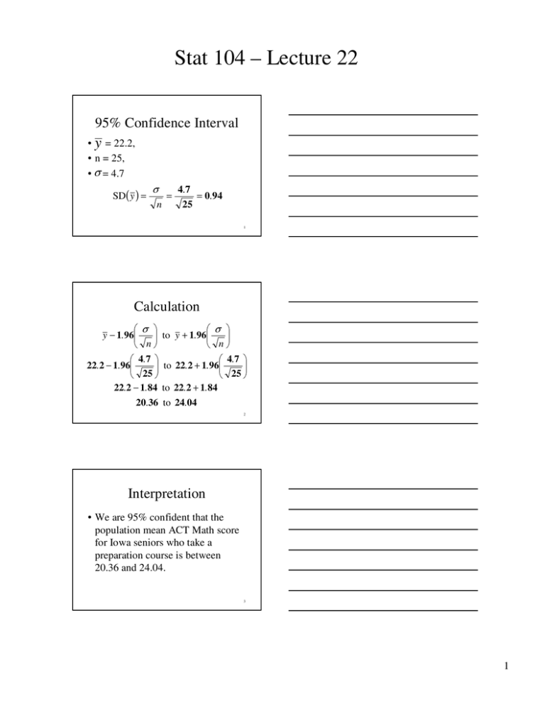
Stat 104 – Lecture 22
95% Confidence Interval
• y = 22.2,
• n = 25,
• σ = 4.7
σ
SD( y ) =
n
=
4.7
= 0.94
25
1
Calculation
⎛
y − 1.96⎜
⎝
σ
n
⎞
⎟
⎠
⎛
to y + 1.96⎜
⎝
σ
n
⎞
⎟
⎠
4.7 ⎞
⎛ 4.7 ⎞
⎟ to 22.2 + 1.96⎜
⎟
⎝ 25 ⎠
⎝ 25 ⎠
22.2 − 1.84 to 22.2 + 1.84
20.36 to 24.04
⎛
22.2 − 1.96⎜
2
Interpretation
• We are 95% confident that the
population mean ACT Math score
for Iowa seniors who take a
preparation course is between
20.36 and 24.04.
3
1
Stat 104 – Lecture 22
How will I use the CI?
• The population mean ACT Math
score for Iowa seniors who take a
preparation course could be any
value between 20.36 and 24.04.
4
95% confidence?
• We have confidence in the procedure
that produces a confidence interval.
• If we repeat that procedure, 95% of
intervals produced will capture the
population mean.
5
95% Confidence?
• Simulation illustrating repeating
the procedure.
• http://statweb.calpoly.edu/chance/a
pplets/ConfSim/ConfSim.html
6
2
Stat 104 – Lecture 22
7
Confidence Level
Confidence
Level
80% 90% 95% 98% 99%
z*
1.28 1.65 1.96 2.33 2.58
8
General Formula
y − z * (SD( y )) to y + z * (SD( y ))
⎛
y − z* ⎜
⎝
σ
n
⎞
⎟
⎠
⎛
to y + z * ⎜
⎝
σ
n
⎞
⎟
⎠
9
3
Stat 104 – Lecture 22
Example
• A random sample of 50 hogs is
taken at a large processing plant.
• The sample mean hot carcass
weight is 187.5 lbs.
10
Example
• Estimate, with 98% confidence, the
population mean hot carcass weight
of all hogs at the processing plant
where the standard deviation of
weights is
σ = 26.1 lbs.
11
Example
⎛
y − z* ⎜
⎝
σ
n
⎞
⎟
⎠
⎛ 26.1 ⎞
⎟
⎝ 50 ⎠
187.5 − 2.33⎜
⎛
to y + z * ⎜
⎝
σ
n
⎞
⎟
⎠
⎛ 26.1 ⎞
⎟
⎝ 50 ⎠
to 187.5 + 2.33⎜
187.5 − 8.6 to 187.5 + 8.6
179.9 to 196.1
12
4