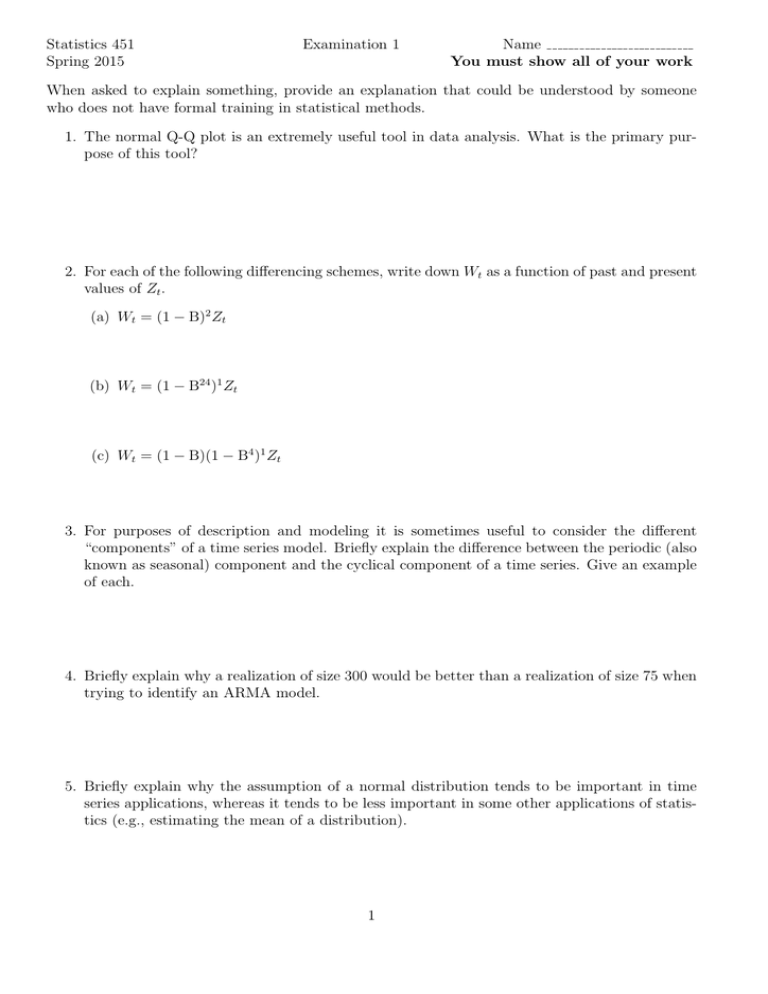
Statistics 451
Spring 2015
Examination 1
Name
You must show all of your work
When asked to explain something, provide an explanation that could be understood by someone
who does not have formal training in statistical methods.
1. The normal Q-Q plot is an extremely useful tool in data analysis. What is the primary purpose of this tool?
2. For each of the following differencing schemes, write down Wt as a function of past and present
values of Zt .
(a) Wt = (1 − B)2 Zt
(b) Wt = (1 − B24 )1 Zt
(c) Wt = (1 − B)(1 − B4 )1 Zt
3. For purposes of description and modeling it is sometimes useful to consider the different
“components” of a time series model. Briefly explain the difference between the periodic (also
known as seasonal) component and the cyclical component of a time series. Give an example
of each.
4. Briefly explain why a realization of size 300 would be better than a realization of size 75 when
trying to identify an ARMA model.
5. Briefly explain why the assumption of a normal distribution tends to be important in time
series applications, whereas it tends to be less important in some other applications of statistics (e.g., estimating the mean of a distribution).
1
6. Consider the following MA time series model
Zt = θ0 + (1 − θ1 B1 )at ,
at ∼ nid(0, σa2 ).
(a) Derive an expression for the mean of Zt .
(b) Derive an expression for the variance of Zt .
(c) Derive expressions for ρ1 , ρ2 , and ρ3 , the autocorrelation between observations separated
by one, two, and three time periods.
(d) Give expressions, as simple as possible, for computing the first three lags of the PACF
function for this MA model.
(e) Find the root(s) of the model-defining polynomial.
(f) For what values of θ1 is the model for Zt invertible? Why?
(g) Is the model for Zt weakly stationary or not? Why or why not?
2
7. The following figure shows monthly data on the number of armed robberies in Boston from
January 1966 to October 1975.
300
100
200
Number
400
500
Number of Armed Robberies in Boston
1966
1967
1968
1969
1970
1971
1972
1973
1974
1975
1976
Time
The following models were fit to the data
Model 1: Yt = β0 + β1 Time + at
Model 2: Yt = β0 + β1 Time + β2 Aug + β3 Dec + · · · + β12 Sep + at
at ∼ nid(0, σa2 )
where Yt is the number of robberies, Time is been defined as (1966.00, 1966.08333, . . . , 1975.75)
and Aug is 1 in August and 0 otherwise, Dec is 1 in month December and 0 otherwise,. . . ,
Sep is 1 in month September and 0 otherwise (there is no dummy variable for April in this
model). The results of the regression fit using ordinary least squares for Model 1 showed
βb0 = −82887, βb1 = 42.15, σ
ba = 44.39 (116 degrees of freedom) and for Model 2, βb0 =
−82561, βb1 = 41.98, βb2 = 57.41, . . . βb12 = 35.11, σ
ba = 41.47 (105 degrees of freedom).
(a) What is the practical interpretation of the parameter β1 in Model 1? (That is, how
would you explain the meaning to someone who did not know much statistics, using the
appropriate units of the coefficient?)
(b) What is the practical interpretation of the parameter β2 in Model 2?
3
(c) What is the practical interpretation of the parameter σa in Model 1?
(d) Explain why there really is no “practical” interpretation for β0 in these models, for this
application.
(e) Compare the results from fitting Models 1 and 2, assuming that at ∼ nid(0, σa2 ). Is there
evidence of a seasonal effect in the data?
(f) The following figure shows the ACF of the residuals from Model 1.
-0.2
0.0
0.2
ACF
0.4
0.6
0.8
1.0
Series : residuals(boston.robberies.fit1)
0
5
10
Lag
15
20
What does this plot tell us about our model assumptions?
(g) How would the value of βb1 change if Time had, instead, been defined as (1, 2, 3, . . . , 118).
4