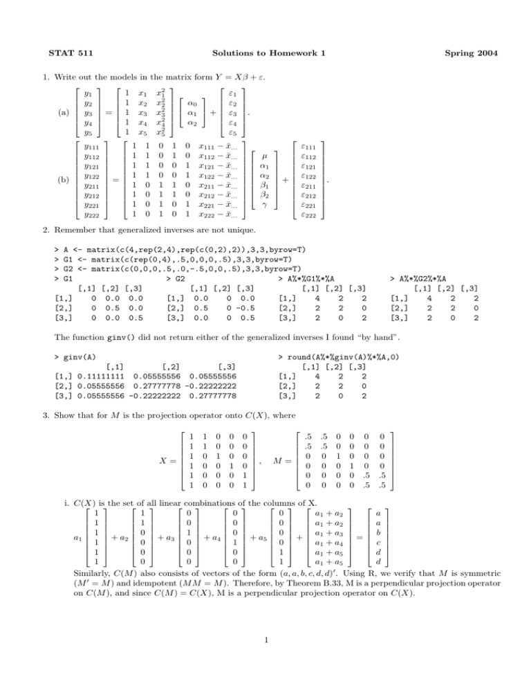
STAT 511
Solutions to Homework 1
1. Write out the models in the matrix form Y = Xβ + ε.
 




y1
1 x1 x21 
ε1

 y2   1 x2 x22  α0
 ε2 

 



2 




ε3 
(a)  y3  =  1 x3 x3  α1 + 

.
 y4   1 x4 x24  α2
 ε4 
y5
1 x5 x25
ε5
 


y111
1 1 0 1 0 x111 − x̄... 
 y112   1 1 0 1 0 x112 − x̄... 
µ

 

 y121   1 1 0 0 1 x121 − x̄...   α1
 


 y122   1 1 0 0 1 x122 − x̄...   α2
=

(b) 
 y211   1 0 1 1 0 x211 − x̄...   β1
 


 y212   1 0 1 1 0 x212 − x̄...   β2

 

 y221   1 0 1 0 1 x221 − x̄... 
γ
y222
1 0 1 0 1 x222 − x̄...
2. Remember that generalized inverses are not unique.




 
 
 
+
 
 
 


ε111
ε112
ε121
ε122
ε211
ε212
ε221
ε222
Spring 2004






.





>
>
>
>
A <- matrix(c(4,rep(2,4),rep(c(0,2),2)),3,3,byrow=T)
G1 <- matrix(c(rep(0,4),.5,0,0,0,.5),3,3,byrow=T)
G2 <- matrix(c(0,0,0,.5,.0,-.5,0,0,.5),3,3,byrow=T)
G1
> G2
> A%*%G1%*%A
[,1] [,2] [,3]
[,1] [,2] [,3]
[,1] [,2] [,3]
[1,]
0 0.0 0.0
[1,] 0.0
0 0.0
[1,]
4
2
2
[2,]
0 0.5 0.0
[2,] 0.5
0 -0.5
[2,]
2
2
0
[3,]
0 0.0 0.5
[3,] 0.0
0 0.5
[3,]
2
0
2
> A%*%G2%*%A
[,1] [,2] [,3]
[1,]
4
2
2
[2,]
2
2
0
[3,]
2
0
2
The function ginv() did not return either of the generalized inverses I found “by hand”.
> ginv(A)
> round(A%*%ginv(A)%*%A,0)
[,1] [,2] [,3]
[1,]
4
2
2
[2,]
2
2
0
[3,]
2
0
2
[,1]
[,2]
[,3]
[1,] 0.11111111 0.05555556 0.05555556
[2,] 0.05555556 0.27777778 -0.22222222
[3,] 0.05555556 -0.22222222 0.27777778
3. Show that for M is the projection operator onto C(X), where




X =



1
1
1
1
1
1
1
1
0
0
0
0
0
0
1
0
0
0
0
0
0
1
0
0
0
0
0
0
1
1





M =






,



.5 .5 0 0 0 0
.5 .5 0 0 0 0
0 0 1 0 0 0
0 0 0 1 0 0
0 0 0 0 .5 .5
0 0 0 0 .5 .5








i. C(X)
 isthe set of all
 linear
 combinations

 of the columns

 ofX.
 

1
1
0
0
0
a1 + a 2
a
 1 
 1 
 0 
 0 
 0   a1 + a 2   a 




 



 
 

 1 
 0 
 1 
 0 
 0   a1 + a 3   b 














a1 
 + a 2  0  + a 3  0  + a 4  1  + a 5  0  +  a1 + a 4  =  c 
 1 


 



 
 

 1 
 0 
 0 
 0 
 1   a1 + a 5   d 
1
0
0
0
1
a1 + a 5
d
0
Similarly, C(M ) also consists of vectors of the form (a, a, b, c, d, d) . Using R, we verify that M is symmetric
(M 0 = M ) and idempotent (M M = M ). Therefore, by Theorem B.33, M is a perpendicular projection operator
on C(M ), and since C(M ) = C(X), M is a perpendicular projection operator on C(X).
1
> X <- matrix(c(rep(1,8),rep(c(rep(0,6),1),3),1),6,5)
> M <- matrix(c(rep(c(.5,.5,0,0,0,0),2),0,0,1,rep(0,6),1,rep(0,6),.5,.5,rep(0,4),.5,.5),6,6,byrow=
> t(M)
> M%*%M
[,1] [,2] [,3] [,4] [,5] [,6]
[,1] [,2] [,3] [,4] [,5] [,6]
[1,] 0.5 0.5
0
0 0.0 0.0
[1,] 0.5 0.5
0
0 0.0 0.0
[2,] 0.5 0.5
0
0 0.0 0.0
[2,] 0.5 0.5
0
0 0.0 0.0
[3,] 0.0 0.0
1
0 0.0 0.0
[3,] 0.0 0.0
1
0 0.0 0.0
[4,] 0.0 0.0
0
1 0.0 0.0
[4,] 0.0 0.0
0
1 0.0 0.0
[5,] 0.0 0.0
0
0 0.5 0.5
[5,] 0.0 0.0
0
0 0.5 0.5
[6,] 0.0 0.0
0
0 0.5 0.5
[6,] 0.0 0.0
0
0 0.5 0.5
?i. [Another choice to show C(X) = C(M )]. Let X = (X 1 , . . . , X 5 ) and M = (M 1 , . . . , M 6 ). Note that every
column in X can be written as a linear combination of columns in M . Therefore, C(X) = C(M ).
P
X1 = 5i=1 Mi , X2 = M1 + M2 , X3 = M3 , X4 = M4 , X5 = M5 + M6 and
M1 = 21 X2 , M2 = 12 X2 , M3 = X3 , M4 = X4 , M5 = 21 X5 , M6 = 12 X5 .
ii. We compute PX = X(X 0 X)− X 0 which is the projection operator onto C(X) and, it matches the matrix
proposed in the statement of this question.
> Px <- X%*%ginv(t(X)%*%X)%*%t(X)
> round(Px,1)
[,1] [,2] [,3] [,4] [,5] [,6]
[1,] 0.5 0.5
0
0 0.0 0.0
[2,] 0.5 0.5
0
0 0.0 0.0
[3,] 0.0 0.0
1
0 0.0 0.0
[4,] 0.0 0.0
0
1 0.0 0.0
[5,] 0.0 0.0
0
0 0.5 0.5
[6,] 0.0 0.0
0
0 0.5 0.5
4. For the same X as in question 3, suppose that Y = (2, 1, 4, 6, 3, 5)0.
(a) Let G1 and G2

0 0.0
 0 0.5

G1 = 
 0 0.0
 0 0.0
0 0.0
be two
0 0
0 0
1 0
0 1
0 0
different generalized inverses for (X 0 X), and let bi


0.0
0.12 −0.02
0.08
0.08
 −0.02
0.0 
0.42
−0.18
−0.18



0.0 
0.72 −0.28
 , G2 =  0.08 −0.18
 0.08 −0.18 −0.28
0.0 
0.72
0.5
−0.02 −0.08 −0.18 −0.18
= Gi X 0 Y for i = 1, 2.

−0.02
−0.08 

−0.18 
.
−0.18 
0.42
Note that Ŷ = Xbi = (1.5, 1.5, 4, 6, 4, 4)0 for i = 1, 2; but b1 = (0, .5, 4, 6, 4)0 and b2 = (3.1, −1.6, 0.9, 2.9, 0.9)0.
(b) >
>
>
>
X <- matrix(c(rep(1,8),rep(c(rep(0,6),1),3),1),6,5)
Y <- c(2,1,4,6,3,5)
Px <- X%*%ginv(t(X)%*%X)%*%t(X)
Yhat <- Px%*%Y
i.
ii.
iii.
iv.
v.
vi.
Ŷ = (1.5, 1.5, 4, 6, 4, 4)0.
Y − Ŷ = (0.5, −0.5, 0, 0, −1, 1)0.
Ŷ 0 (Y − Ŷ ) = 0.
Y 0 Y = 91.
Ŷ 0 Ŷ = 88.5.
(Y − Ŷ )0 (Y − Ŷ ) = 2.5.


3 0 −1
0 .
5. Let Y = (y1 , y2 , y3 )0 with Y N (µ, V ) where µ = (0, 1, 0)0 and V =  0 5
−1 0 10
(a) y3 ∼ N (0, 10).
y1
0
3 −1
(b)
∼N
,
.
y3
0
−1 10
(c) y3 |y1 = 2 ∼ N (−2/3, 29/3).
2
(d)
y3 |y1 = 2, y2 = −1 ∼ N
(e)
y1
y3
=
−1
y2
0+
−1 0
3 0
0 5
−1 2−0
−1 − 1
, 10 −
−1 0
3 0
0 5
−1 −1
0
= N (−2/3, 29/3) f (y3 |y1 , y2 ) = f (y3 |y1 ).
0
0
3 −1
0
∼ N
+
[1/5][−1 − 1],
−
[1/5] 0 0
−1 10
0
0 0
.
0
3 −1
= N
,
f (y1 , y3 |y2 ) = f (y1 , y3 )
0
−1 10
!
(f) Find the correlations ρ12 , ρ13 , ρ23
p
i. ρ12 = 0/ 3(5) = 0.
p
√
ii. ρ13 = −1/ 3(10) = −1/ 30.
p
iii. ρ23 = 0/ 5(10) = 0.



1 3
1
−1
1
0
1
−1
1
−1
16 1




(g) Z ∼ N
E(Y ) +
,
Cov(Y ) −1 1
=N
,
.
3
1 0
1
3 1 0
2
1 32
1 0
6. Using the function eigen() to obtain eigenvalues and eigenvectors of a matrix V we are able to compute its inverse
square root, W = V −1/2 = U D−1/2 U 0 . Note that W W = V −1 .
>
>
>
>
V <- matrix(c(3,-1,1,-1,5,-1,1,-1,3),3,3,byrow=T)
EV <- eigen(V)
W <- EV$vectors%*%diag(1/sqrt(EV$values))%*%t(EV$vectors)
W
[,1]
[,2]
[,3]
[1,] 0.61404486 0.05636733 -0.09306192
[2,] 0.05636733 0.46461562 0.05636733
[3,] -0.09306192 0.05636733 0.61404486
> W%*%W
[,1]
[,2]
[,3]
[1,] 0.38888889 0.05555556 -0.11111111
[2,] 0.05555556 0.22222222 0.05555556
[3,] -0.11111111 0.05555556 0.38888889
> solve(V)
[,1]
[,2]
[,3]
[1,] 0.38888889 0.05555556 -0.11111111
[2,] 0.05555556 0.22222222 0.05555556
[3,] -0.11111111 0.05555556 0.38888889
7. > A <- matrix(c(4,4.001,4.001,4.002),2,2)
> B <- matrix(c(4,4.001,4.001,4.002001),2,2)
> det(A);det(B)
# determinants of A and B, respectively.
[1] -1e-06
# 4*4.002-4.001*4.001
[1] 3e-06
# 4*4.002001-4.001*4.001
> ginv(A)
[,1]
[,2]
[1,] -4002000 4001000
[2,] 4001000 -4000000
> ginv(B)
[,1]
[,2]
[1,] 1334000 -1333667
[2,] -1333667 1333333
> 3*ginv(B)
[,1]
[,2]
[1,] 4002001 -4001000
[2,] -4001000 4000000
3