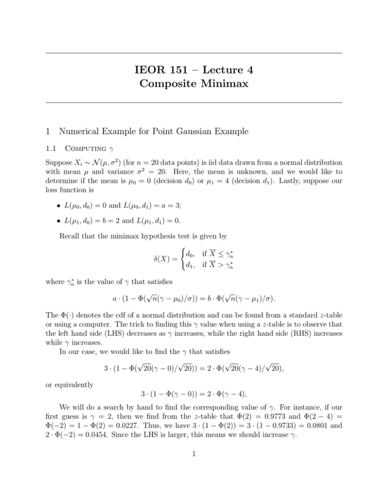
IEOR 151 – Lecture 4
Composite Minimax
1 Numerical Example for Point Gaussian Example
1.1
Computing γ
Suppose Xi ∼ N (µ, σ 2 ) (for n = 20 data points) is iid data drawn from a normal distribution
with mean µ and variance σ 2 = 20. Here, the mean is unknown, and we would like to
determine if the mean is µ0 = 0 (decision d0 ) or µ1 = 4 (decision d1 ). Lastly, suppose our
loss function is
• L(µ0 , d0 ) = 0 and L(µ0 , d1 ) = a = 3;
• L(µ1 , d0 ) = b = 2 and L(µ1 , d1 ) = 0.
Recall that the minimax hypothesis test is given by
(
d0 , if X ≤ γn∗
δ(X) =
d1 , if X > γn∗
where γn∗ is the value of γ that satisfies
√
√
a · (1 − Φ( n(γ − µ0 )/σ)) = b · Φ( n(γ − µ1 )/σ).
The Φ(·) denotes the cdf of a normal distribution and can be found from a standard z-table
or using a computer. The trick to finding this γ value when using a z-table is to observe that
the left hand side (LHS) decreases as γ increases, while the right hand side (RHS) increases
while γ increases.
In our case, we would like to find the γ that satisfies
√
√
√
√
3 · (1 − Φ( 20(γ − 0)/ 20)) = 2 · Φ( 20(γ − 4)/ 20),
or equivalently
3 · (1 − Φ(γ − 0)) = 2 · Φ(γ − 4),
We will do a search by hand to find the corresponding value of γ. For instance, if our
first guess is γ = 2, then we find from the z-table that Φ(2) = 0.9773 and Φ(2 − 4) =
Φ(−2) = 1 − Φ(2) = 0.0227. Thus, we have 3 · (1 − Φ(2)) = 3 · (1 − 0.9733) = 0.0801 and
2 · Φ(−2) = 0.0454. Since the LHS is larger, this means we should increase γ.
1
Now suppose our second guess is γ = 2.5. Then, Φ(2.5) = 0.9938 and Φ(2.5 − 4) =
Φ(−1.5) = 1 − Φ(1.5) = 1 − 0.9332. Thus, we have that LHS = 3 · (1 − 0.9938) = 0.0186
and RHS = 2 · (1 − 0.9332) = 0.1336. Now, the RHS is larger and so we should decrease our
guess of γ. Since we know that γ = 2 is too small, we could try half-way in between with
γ = 2.25.
We can summarize the steps We conclude the process when we have sufficient accuracy
Step
1
2
3
4
5
6
7
8
γ
2
2.5
2.25
2.13
2.06
2.09
2.07
2.08
LHS
0.0801
0.0186
0.0367
0.0498
0.0591
0.0549
0.0577
0.0563
RHS
0.0454
0.1336
0.0801
0.0615
0.0524
0.0561
0.0536
0.0549
in our computed value of γ. In this case, we know that γ should be between 2.08 and 2.09,
and so we set γn∗ = 2.085. Computing γ to more precision would require a computer.
1.2
Differences in γ as n Changes
In the above example, we computed γn∗ for a single value of n = 20. A natural question
to ask is what happens to γ as n increase. In the table below, the value of γn∗ for different
values of n is given. These values were computed using a computer.
n
5
10
20
100
200
300
γn∗
2.2658
2.1536
2.0855
2.0194
2.0099
2.0068
The trend is clear: As n increases, γn∗ is decreasing towards 2. The intuition is that when
we have little data, we err on the side of deciding d0 since otherwise we incur a larger loss
if we incorrectly decide d1 . As we gather more data, we are more confident that the sample
average is close to the true average, and so we can use a less biased threshold. Effectively,
with large amounts of data the threshold converges to (µ0 + µ1 )/2.
2 Composite Gaussian Example
In our discussion so far, we have considered a situation in which the two hypothesis each
represent a distribution with a single mean. However, another class of interesting and more
2
general hypotheses are those in which we would like to discrimination between H0 : µ ≤
µ0 versus H1 : µ > µ0 . And suppose we keep a similar loss function of L(H0 , d0 ) = 0,
L(H0 , d1 ) = a, L(H1 , d0 ) = b, and L(H1 , d1 ) = 0. In the minimax framework, this class of
hypotheses are not well-posed because the worst case scenario occurs when “nature” selects
µ = µ0 , because then it is not possible to distinguish between d0 and d1 .
More rigorously, what happens is that the minimax procedure is defined by solving the
optimization problem
inf sup R(µ, δ).
δ(u)
µ
And nature will choose
sup R(µ, δ) = sup a · Pµ (d1 = δ(X))}
µ:µ≤µ0
µ:µ≤µ0
= a · Pµ0 (d1 = δ(X))}
and
sup R(µ, δ) = sup b · Pµ (d0 = δ(X))}
µ:µ>µ0
µ:µ>µ0
= b · Pµ0 (d0 = δ(X))}.
This last step is subtle: Even though nature is constrained to choose µ > µ0 , it can choose
µ to be arbitarily close to µ0 . Thus, in the worst case scenario described by the minimax
framework, nature will effectively set µ = µ0 even though we are in the case H1 : µ > µ0 .
Because of this pathological behavior, the best we can do with a minimax procedure is
to make a purely probabilistic decision:
(
d0 , with probability a/(a + b)
δ(X) =
d1 w.p. b/(a + b)
This is not a useful rule for decision making, and so we must consider alternative classes of
hypotheses.
One interesting class of hypotheses is the following: Suppose X1 , . . . , Xn ∼ N (µ, σ 2 ) is
iid data drawn from a normal distribution with mean µ and known variance σ 2 ; here, the
mean is unknown. The decision we would like to make is whether the mean is H0 : µ ≤ µ0
or H1 : µ ≥ µ1 . We are indifferent in the case where I : µ ∈ (µ0 , µ1 ). Our loss function also
encodes this region of indifference
• L(H0 , d0 ) = 0, L(H0 , d1 ) = a;
• L(H1 , d0 ) = b, L(H1 , d1 ) = 0;
• L(I, d0 ) = 0, L(I, d1 ) = 0.
3
It turns out that this composite hypothesis test has the same minimax procedure as the
point hypothesis test. To summarize, we choose γ so that it satisfies
√
√
a · (1 − Φ( n(γ − µ0 )/σ)) = b · Φ( n(γ − µ1 )/σ),
where Φ(·) is the cdf of a normal distribution. If we call this resulting value γ ∗ , then our
decision rule is
(
d0 , if X ≤ γ ∗
δ(X) =
d1 , if X > γ ∗
Showing that this decision rule is a minimax procedure is beyond the scope of the class.
4